Wrap Up
Contents
Wrap Up#
1. Installing Python packages#
Install packages in a Jupyter notebook on any machine, including your own! (And if you don’t have Python and Jupyter notebooks installed on your computer you can find instructions to install them here. The following cell will install the three packages we have been using all semester:
!pip3 install -q cs104@git+https://github.com/cs104williams/cs104-toolbox
!pip3 install -q datascience@git+https://github.com/cs104williams/cs104-datascience
!pip3 install -q numpy
We import packages that have been installed in order to use their features in our code:
# Second step: import packages
from datascience import *
from cs104 import *
import numpy as np
%matplotlib inline
Now let’s install three different packages we haven’t seen yet…
!pip3 install -q pandas
!pip3 install -q scikit-learn
!pip3 install -q seaborn
import pandas as pd
from sklearn import *
import matplotlib.pyplot as plots
import seaborn as sns
2. Pandas#
Pandas is a library to manipulate and explore data (similar to Tables), but with more functionality.
penguins = pd.read_csv('https://raw.githubusercontent.com/mcnakhaee/palmerpenguins/master/palmerpenguins/data/penguins.csv')
penguins = penguins.drop(columns = ['year'])
penguins.head(6)
| species | island | bill_length_mm | bill_depth_mm | flipper_length_mm | body_mass_g | sex | |
|---|---|---|---|---|---|---|---|
| 0 | Adelie | Torgersen | 39.1 | 18.7 | 181.0 | 3750.0 | male |
| 1 | Adelie | Torgersen | 39.5 | 17.4 | 186.0 | 3800.0 | female |
| 2 | Adelie | Torgersen | 40.3 | 18.0 | 195.0 | 3250.0 | female |
| 3 | Adelie | Torgersen | NaN | NaN | NaN | NaN | NaN |
| 4 | Adelie | Torgersen | 36.7 | 19.3 | 193.0 | 3450.0 | female |
| 5 | Adelie | Torgersen | 39.3 | 20.6 | 190.0 | 3650.0 | male |
# pandas gives us a quick summary of the data
penguins.info()
<class 'pandas.core.frame.DataFrame'>
RangeIndex: 344 entries, 0 to 343
Data columns (total 7 columns):
 #   Column             Non-Null Count  Dtype
---  ------             --------------  -----
 0   species            344 non-null    object
 1   island             344 non-null    object
 2   bill_length_mm     342 non-null    float64
 3   bill_depth_mm      342 non-null    float64
 4   flipper_length_mm  342 non-null    float64
 5   body_mass_g        342 non-null    float64
 6   sex                333 non-null    object
dtypes: float64(4), object(3)
memory usage: 18.9+ KB
penguins = penguins.dropna()
penguins.head(6)
| species | island | bill_length_mm | bill_depth_mm | flipper_length_mm | body_mass_g | sex | |
|---|---|---|---|---|---|---|---|
| 0 | Adelie | Torgersen | 39.1 | 18.7 | 181.0 | 3750.0 | male |
| 1 | Adelie | Torgersen | 39.5 | 17.4 | 186.0 | 3800.0 | female |
| 2 | Adelie | Torgersen | 40.3 | 18.0 | 195.0 | 3250.0 | female |
| 4 | Adelie | Torgersen | 36.7 | 19.3 | 193.0 | 3450.0 | female |
| 5 | Adelie | Torgersen | 39.3 | 20.6 | 190.0 | 3650.0 | male |
| 6 | Adelie | Torgersen | 38.9 | 17.8 | 181.0 | 3625.0 | female |
print('num rows (after droping nulls) = ', len(penguins))
num rows (after droping nulls) = 333
penguins[penguins.species == 'Adelie'].mean(numeric_only=True)
bill_length_mm         38.823973
bill_depth_mm          18.347260
flipper_length_mm     190.102740
body_mass_g          3706.164384
dtype: float64
3. Seaborn#
Seaborn is a Data visualization library. Interfaces with pandas nicely. Makes very pretty plots!
# The cs104 library changes the default plot settings.
# This line changes them back
sns.set_theme()
sns.scatterplot(penguins, x="bill_length_mm", y="bill_depth_mm", hue="species");
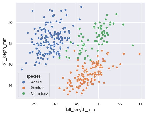
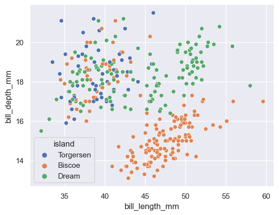
A big advantage of seaborn is that you can quickly visualize different subsets of data:
sns.scatterplot(penguins, x="bill_length_mm", y="bill_depth_mm", hue="island");
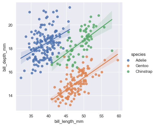
sns.lmplot(penguins, x="bill_length_mm", y="bill_depth_mm", hue="species");
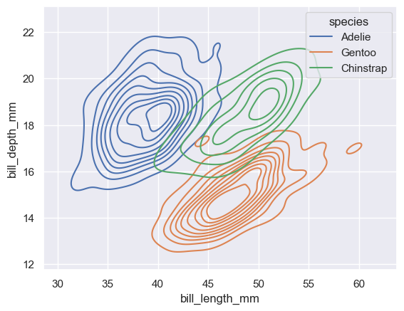
sns.kdeplot(penguins, x="bill_length_mm", y="bill_depth_mm", hue="species");
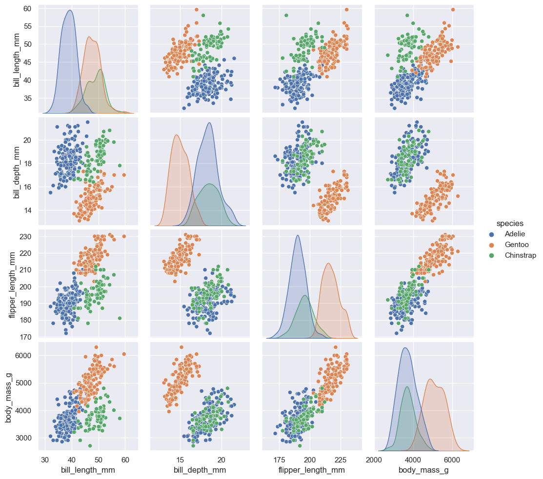
sns.pairplot(penguins, hue="species");
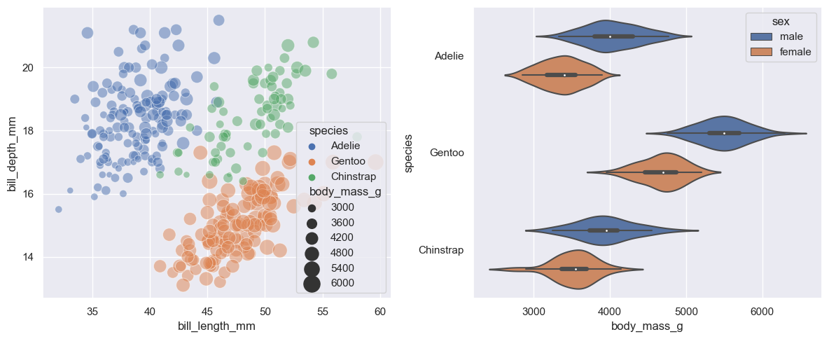
fig, ax = plots.subplots(1,2,figsize=(12,5))
sns.scatterplot(penguins, x="bill_length_mm", y="bill_depth_mm", hue="species",
                size="body_mass_g", sizes=(30, 300), alpha=0.5,
                ax=ax[0])
sns.violinplot(penguins, x="body_mass_g", y="species", hue="sex",
               ax=ax[1])
fig.tight_layout()
4. sklearn (Scikit-Learn)#
sklearn — pronounced Sci Kit Learn — is a library for machine learning (statistical pattern matching).
Linear Regression with sklearn#
from sklearn import linear_model

from sklearn.metrics import r2_score as r2_score_sklearn
from sklearn.metrics import mean_squared_error as mse_sklearn
from sklearn.feature_selection import r_regression
# Some data wrangling to get our x and y values, this time with pandas...
chinstrap = penguins[penguins['species'] == 'Chinstrap']
x = chinstrap['bill_length_mm'].to_numpy().reshape(-1, 1)
y = chinstrap['bill_depth_mm'].to_numpy()
model = linear_model.LinearRegression()
model.fit(x, y)
LinearRegression()In a Jupyter environment, please rerun this cell to show the HTML representation or trust the notebook.
On GitHub, the HTML representation is unable to render, please try loading this page with nbviewer.org.
LinearRegression()
print('slope    ', model.coef_[0])
print('intercept', model.intercept_)
slope     0.2222117240036715
intercept 7.569140119132472
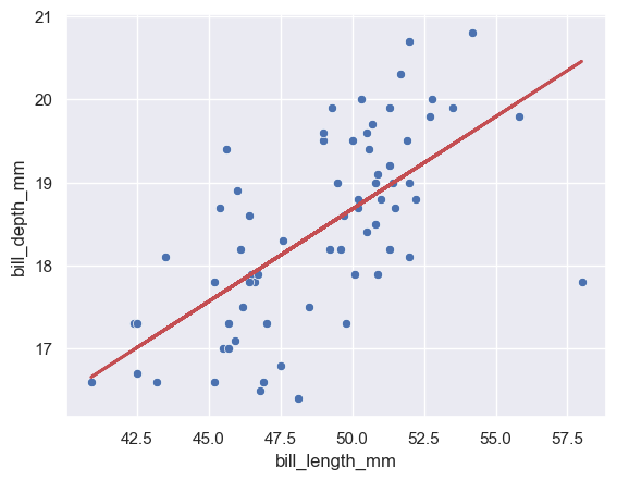
y_hat = model.predict(x)
sns.scatterplot(chinstrap, x='bill_length_mm', y='bill_depth_mm')
plots.plot(x, y_hat, color='r', lw=2);
A whole lot of metrics we might want are already implemented in sklearn.
print('Pearson Correlation:', r_regression(x, y)[0])
print('MSE:                ', mse_sklearn(y, y_hat))
print('R2 Score:           ', r2_score_sklearn(y, y_hat))
Pearson Correlation: 0.653536208180049
MSE:                 0.7276649994299124
R2 Score:            0.4271095754023476
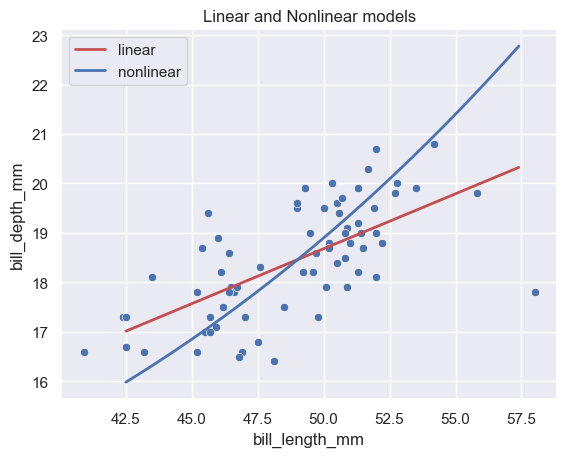
Non-linear Regresion#
New: let’s fit a non-linear regression line with sklearn!
model_nonlinear = svm.SVR(kernel='poly') #does non-linear (polynomial) regression
model_nonlinear.fit(x, y)
SVR(kernel='poly')In a Jupyter environment, please rerun this cell to show the HTML representation or trust the notebook.
On GitHub, the HTML representation is unable to render, please try loading this page with nbviewer.org.
SVR(kernel='poly')
# plot what the polynomial regression does
x_range = np.arange(42.5, 57.5, 0.1).reshape(-1, 1)

y_hat_linear = model.predict(x_range)
y_hat_nonlinear = model_nonlinear.predict(x_range)

sns.scatterplot(chinstrap, x='bill_length_mm', y='bill_depth_mm')
plots.plot(x_range, y_hat_linear, color='r', label='linear', lw=2);
plots.plot(x_range, y_hat_nonlinear, color='b', label='nonlinear', lw=2)
plots.title("Linear and Nonlinear models")
plots.legend();
Take Machine Learning to learn the process for evaluating which model is better!