Inference Library Reference#

  • Click on any row to see detailed examples.

Library Sections

Sampling and Simulation

Name Description Parameters Output

sample_proportions(sample_size,        
                   model_proportions)

Sample_size should be an integer, model_proportions an array of probabilities that sum up to 1. The function samples sample_size objects from the distribution specified by model_proportions. It returns an array with the same size as model_proportions. Each item in the array corresponds to the proportion of times it was sampled out of the sample_size times.

  1. int : sample size

  2. array : an array of proportions that should sum to 1

array : each item corresponds to the proportion of times that corresponding item was sampled from model_proportions in sample_size draws, should sum to 1

Examples
model_proportions = make_array(0.9, 0.1)
sample_proportions(100, model_proportions)
array([0.91, 0.09])
model_proportions = make_array(0.7, 0.2, 0.1)
sample_proportions(100, model_proportions)
array([0.71, 0.2 , 0.09])

simulate(make_one_outcome, num_outcomes)

Simulates the outcome of num_outcomes events. The outcome of an event is computed by the make_one_outcome function passed to simulate

  • make_one_outcome: a function that returns the outcome of an event.

  • num_outcomes: the number of events to simulate.

An array of the simulated outcomes.

Examples
dice = np.arange(1,7)

def roll_two_dice():
  return np.random.choice(dice) + np.random.choice(dice)
simulate(roll_two_dice, 10)
array([12.,  3.,  4., 11.,  8., 10.,  7., 10.,  8.,  8.])

simulate_sample_statistic(make_one_sample,
   sample_size,
   compute_statistic,
   num_trials)

Simulates the process of computing a statistic for random samples.

  • make_one_sample: a function that takes an int \(n\) and returns a sample as an array of \(n\) elements.

  • sample_size: the size of the samples to use in the simulation.

  • compute_statistic: a function that takes a sample as an array and returns the statistic for that sample.

  • num_trials: the number of simulation steps to perform.

An array of the simulated statistics.

Examples
coin = make_array('heads', 'tails')

def flip_coins(n):
  return np.random.choice(coin, n)

def count_heads(sample):
  return np.count_nonzero(sample == 'heads')

simulate_sample_statistic(flip_coins, 100, 
                          count_heads, 10)
array([53., 53., 49., 53., 55., 60., 52., 46., 52., 54.])
coin = make_array('heads', 'tails')

def flip_coins(n):
  return np.random.choice(coin, n)

def diff_from_half_heads(sample):
  return abs(np.count_nonzero(sample == 'heads') - len(sample)/2)

simulate_sample_statistic(flip_coins, 100, 
                          diff_from_half_heads, 10)
array([5., 2., 5., 5., 6., 1., 5., 2., 3., 2.])

Hypothesis Testing

Name Description Parameters Output

empirical_pvalue(simulated_statistics,
    observed_statistic)

Computes the proportion of values in simulated statistics that are at least as large as observed_statistic

  • simulated_statistics: an array of int of float.

  • observed_statistic: an int or float.

A proportion.

Examples
sample_statistics = make_array(2,2,3,4,5,2,2,6)
empirical_pvalue(sample_statistics, 5)    
0.25
sample_statistics = make_array(2,2,3,4,5,2,2,6)
empirical_pvalue(sample_statistics, 6)    
0.125

Permutation Tests

Name Description Parameters Output

permutation_sample(table,
    group_label)

Returns the given table augmented with a new column Shuffled Labels that contains a permutation of the values in the column group_column_label.

  • table: a Table.

  • group_label: the column to permute.

A new Table.

Examples
trial
Group Outcome
Control 0
Control 0
Control 1
Control 0
Treatment 1
Treatment 1
Treatment 0
Treatment 1
permutation_sample(trial, 'Group')
Group Outcome Shuffled Label
Control 0 Treatment
Control 0 Control
Control 1 Control
Control 0 Treatment
Treatment 1 Treatment
Treatment 1 Control
Treatment 0 Control
Treatment 1 Treatment

abs_difference_of_means(table,
   group_label,
   value_label)

Takes a table, the label of the column used to divide rows into two groups, and the label of the column storing the values for each row. Returns: the absolute difference of means for the two groups.

Note: If the values are all 0 or 1, then the result can be interpreted as the difference in the proportion of 1 for the two groups.

  • table: a Table.

  • group_label: the column to divide the rows.

  • value_label: the column holding numerical values.

A new Table.

Examples
sizes
Color Size
Blue 2
Blue 4
Red 3
Blue 6
Red 2
Red 1
abs_difference_of_means(sizes, 'Color', 'Size')
2.0
trial
Group Outcome
Control 0
Control 0
Control 1
Control 0
Treatment 1
Treatment 1
Treatment 0
Treatment 1
abs_difference_of_means(trial, 'Group', 'Outcome')
0.5

simulate_permutation_statistic(table,
   group_label,
   value_label,
   num_trials)

Simulates num_trials permutation sampling steps and returns an array of abs_difference_of_means statistics for those samples.

  • table: a Table.

  • group_label: the column to divide the rows.

  • value_label: the column holding the values of interest.

  • num_trials: the number of simulation steps to perform.

An array of the simulated statistics.

Examples
big_trial.sample(10)
Group Outcome
Control 0
Control 0
Treatment 1
Control 0
Treatment 1
Control 0
Control 0
Treatment 1
Treatment 0
Control 0
simulate_permutation_statistic(big_trial, 'Group', 
                               'Outcome', 5)
array([0.006, 0.022, 0.006, 0.034, 0.018])

Bootstrapping and Confidence Intervals

Name Description Parameters Output

bootstrap_statistic(initial_sample,
    compute_statistic,
    num_trials)

Simulates the process of computing a statistic for resamples of one original sample. The original sample is represented as a array, and the compute_statistic function should take in an array.

  • initial_sample: an array representing the sample we start with.

  • compute_statistic: a function that takes a sample as an array and returns the statistic for that sample.

  • num_trials: the number of resampling steps to perform.

An array of the simulated statistics for the resamples.

Examples
observed_sample = make_array(1,2,3,4,5)

bootstrap_statistic(observed_sample, np.mean, 5)
array([4.8, 3.4, 1.8, 3. , 3.4])
statistics = bootstrap_statistic(observed_sample,
                                 np.mean, 2000)

plot = Table().with_columns('bootstrap statistics', 
                            statistics).hist()
plot.dot(np.mean(observed_sample))
../_images/inference-library-ref_39_0.png

confidence_interval(ci_percent,
    statistics)

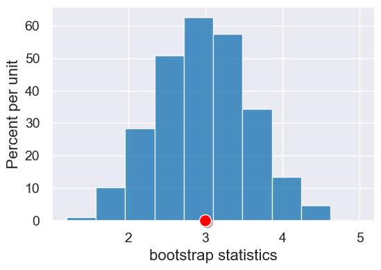
Returns an array with the lower and upper bound of the ci_percent confidence interval.

  • ci_percent: The percent of statistics covered by the confidence interval.

  • statistics: An array of statistics.

An array of two elements.

Examples
observed_sample = make_array(1,2,3,4,5)

statistics = bootstrap_statistic(observed_sample, 
                                 np.mean, 5000)
left, right = confidence_interval(95, 
                                  statistics)
print(left, right)
1.8 4.2
statistics = bootstrap_statistic(observed_sample, 
                                 np.mean, 5000)

plot = Table().with_columns('statistics', 
                            statistics).hist()

ci = confidence_interval(95, statistics)
plot.interval(ci)
plot.dot(np.mean(observed_sample))
../_images/inference-library-ref_43_0.png

Linear Regression

Name Description Parameters Output

pearson_correlation(table,
   x_label, y_label)

Computes the correlation coefficient capturing the sign and strength of the association between the given columns in the table.

  • table: The Table of data.

  • x_label, y_label: Labels of the columns for the x-axis and y-axis.

A float between -1 and 1.

Examples
bills.scatter('bill_length_mm','bill_depth_mm')
../_images/inference-library-ref_45_0.png
pearson_correlation(bills, 'bill_length_mm','bill_depth_mm')
0.3914916918358763

line_predictions(a, b, x)

Computes the prediction y_hat = a * x + b where a and b are the slope and intercept and x is the set of x-values.

  • a, b: Slope and intercept of line

  • x: an array of x values.

an array of predicted y values.

Examples
x = make_array(4,8,12,16)
x
array([ 4,  8, 12, 16])
y_hat = line_predictions(0.25, 3, x)
y_hat
array([4., 5., 6., 7.])
lengths = small_bills.column('bill_length_mm')

lengths
array([39.1, 39.5, 40.3, 36.7, 39.3])
predicted_depths = line_predictions(0.18, 11.4, 
                                    lengths)
predicted_depths
array([18.438, 18.51 , 18.654, 18.006, 18.474])

linear_regression(table,
   x_label, y_label)

Computes the slope and intercept of the line best fitting the table’s data according to the mean square error loss function.

  • table: The Table of data.

  • x_label, y_label: Labels of the columns for the x-axis and y-axis.

A two-element array with the slope and intercept.

Examples
optimal = linear_regression(bills, 'bill_length_mm',
                                   'bill_depth_mm')
a = optimal.item(0)
b = optimal.item(1)
print('a = ', a, '  b = ', b)
a =  0.17883434929831496   b =  11.409124493057005
# a shorcut to assign to a and b all in one line.
a,b = linear_regression(bills, 'bill_length_mm',
                               'bill_depth_mm')

print('a = ', a, '  b = ', b)
a =  0.17883434929831496   b =  11.409124493057005

r2_score(table,
   x_label, y_label,
   a, b)

Given the values \(x\) and \(y\) in the x_label and y_label columns, computes the r-squared score (also called the “coefficient of determination”) for the predictions given \(y=ax+b\).

  • table: The Table of data.

  • x_label, y_label: Labels of the columns for the x-axis and y-axis.

  • a, b: Slope and intercept of line

A float between 0 and 1.

Examples
a,b = linear_regression(bills,'bill_length_mm','bill_depth_mm')
r2_score(bills,'bill_length_mm','bill_depth_mm', a,b)
0.15326574477651644

plot_scatter_with_line(table,
   x_label, y_label,
   a, b)

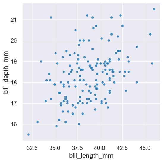
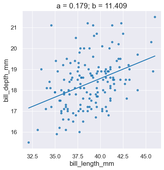
Plots a scatter graph for the points in given columns and also a line for the equation \(y = ax+b\).

  • table: The Table of data.

  • x_label, y_label: Labels of the columns for the x-axis and y-axis.

  • a, b: Slope and intercept of line

A Plot.

Examples
a,b = linear_regression(bills,'bill_length_mm','bill_depth_mm')
plot_scatter_with_line(bills,'bill_length_mm','bill_depth_mm',a,b)
../_images/inference-library-ref_63_0.png

plot_residuals(table,
   x_label, y_label,
   a, b)

Given the values \(x\) and \(y\) in the x_label and y_label columns, plots the residuals \((x, y - \hat{y})\), where \(\hat{y}\) are the predictions from the line characterized by \(y = ax+b\).

  • table: The Table of data.

  • x_label, y_label: Labels of the columns for the x-axis and y-axis.

  • a, b: Slope and intercept of line

A Plot.

Examples
a,b = linear_regression(bills,'bill_length_mm','bill_depth_mm')
with Figure(1,2):
    plot_scatter_with_line(bills,'bill_length_mm','bill_depth_mm',a,b)
    plot_residuals(bills,'bill_length_mm','bill_depth_mm',a,b)
../_images/inference-library-ref_65_0.png

plot_regression_and_residuals(table,
   x_label, y_label,
   a, b)

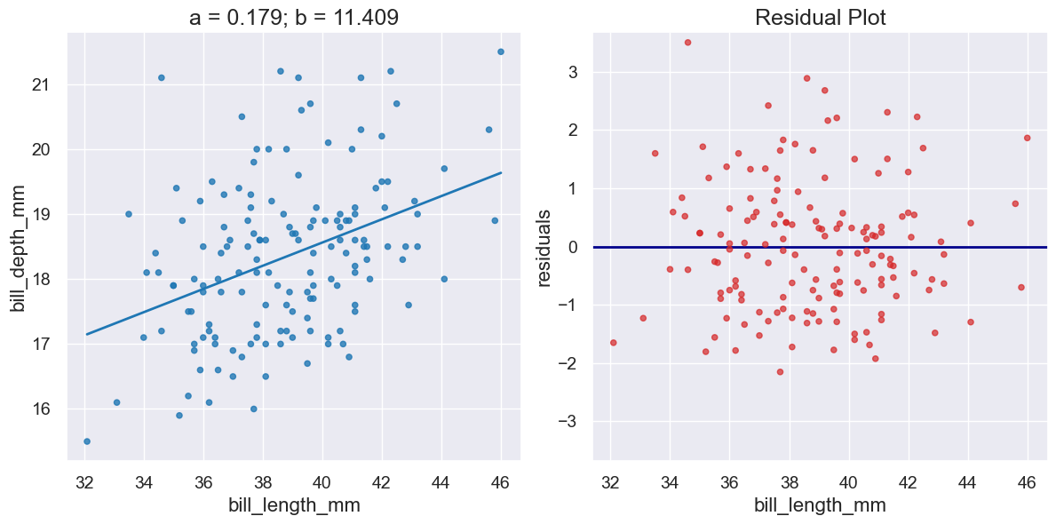
Create a pair of plots capturing 1) a scatter plot and the line \(y=ax+b\) and 2) the residuals when that line is used for preductions. Returns the Plot for the scatter plot.

  • table: The Table of data.

  • x_label, y_label: Labels of the columns for the x-axis and y-axis.

  • a, b: Slope and intercept of line

A Plot.

Examples
a,b = linear_regression(bills,'bill_length_mm','bill_depth_mm')
plot_regression_and_residuals(bills,'bill_length_mm','bill_depth_mm',a,b)
../_images/inference-library-ref_67_0.png