Linear Regression
Contents
Linear Regression#
from datascience import *
from cs104 import *
import numpy as np
%matplotlib inline
/Users/freund/miniconda3/envs/cs104/lib/python3.11/site-packages/datascience/maps.py:13: UserWarning: pkg_resources is deprecated as an API. See https://setuptools.pypa.io/en/latest/pkg_resources.html. The pkg_resources package is slated for removal as early as 2025-11-30. Refrain from using this package or pin to Setuptools<81.
import pkg_resources
Helper functions for visualizations#
This code in the next cell is used in the rest of the notebook to create visualizations. You do not need to look at or understand all the details of it.
import matplotlib.colors as colors
import matplotlib.pyplot as plots
def plot_line(a, b, x):
"""
Plots a line using the give slope and intercept over the
range of x-values in the x array.
"""
xlims = make_array(min(x), max(x))
plot = Plot()
plot.line(xlims, a * xlims + b, lw=4, clip_on=False)
def line_predictions(a, b, x):
"""
Computes the prediction y_hat = a * x + b
where a and b are the slope and intercept and x is the set of x-values.
"""
return a * x + b
def visualize_scatter_with_line_and_residuals(table, x_label, y_label, a, b):
"""
Draw a scatter plot, a line, and the line segments capturing the residuals
for some of the points.
"""
y_hat = line_predictions(a, b, table.column(x_label))
prediction_table = table.with_columns(y_label + '_hat', y_hat)
plot = table.scatter(x_label, y_label, title='a = ' + str(round(a,3)) + '; b = ' + str(round(b,3)))
xlims = make_array(min(table.column(x_label)), max(table.column(x_label)))
plot.line(xlims, a * xlims + b, lw=4, color="C0")
every10th = prediction_table.sort(x_label).take(np.arange(0,
prediction_table.num_rows,
prediction_table.num_rows // 10))
for row in every10th.rows:
x = row.item(x_label)
y = row.item(y_label)
plot.line([x, x], [y, a * x + b], color='r', lw=2)
plot.dot(x,y,color='C0',s=70)
return plot
def mean_squared_error(table, x_label, y_label, a, b):
y_hat = line_predictions(a, b, table.column(x_label))
residual = table.column(y_label) - y_hat
return np.mean(residual**2)
def visualize_scatter_with_line_and_mse(table, x_label, y_label, a, b):
plot = visualize_scatter_with_line_and_residuals(table, x_label, y_label, a, b)
mse = mean_squared_error(x_y_table, x_label, y_label, a, b)
plot.set_title('a = ' + str(round(a,3)) +
'; b = ' + str(round(b,3)) +
'\n mse = ' + str(round(mse,3)))
## MSE HEAT
def plot_regression_line_and_mse_heat(table, x_label, y_label, a, b, show_mse='2d', fig=None):
"""
Left plot: the scatter plot with line y=ax+b
Right plot: None, 2D heat map of MSE, or 3D surface plot of MSE
"""
a_space = np.linspace(-0.5, 0.5, 200)
b_space = np.linspace(-35, -8, 200)
a_space, b_space = np.meshgrid(a_space, b_space)
broadcasted = np.broadcast(a_space, b_space)
mses = np.empty(broadcasted.shape)
mses.flat = [mean_squared_error(table, 'x', 'y', a, b) for (a,b) in broadcasted]
if fig is None:
fig = Figure(1,2)
ax = fig.axes()
#Plot the scatter plot and best fit line on the left
with Plot(ax[0]):
plot_scatter_with_line(table, x_label, y_label, a, b)
if show_mse == '2d':
with Plot(ax[1]):
mse = mean_squared_error(table, x_label, y_label, a, b)
ax[1].pcolormesh(a_space, b_space, mses, cmap='viridis',
norm=colors.PowerNorm(gamma=0.25,
vmin=mses.min(),
vmax=mses.max()));
ax[1].scatter(a,b,s=100,color='red');
ax[1].set_xlabel('a')
ax[1].set_ylabel('b')
ax[1].set_title('Mean Squared Error: ' + str(np.round(mse, 3)))
elif show_mse == "3d":
ax[1] = plots.subplot(1, 2, 2, projection='3d')
with Plot(ax[1]):
ax[1].plot_surface(a_space, b_space, mses,
cmap='viridis',
antialiased=False,
linewidth=0,
norm = colors.PowerNorm(gamma=0.25,vmin=mses.min(), vmax=mses.max()))
ax[1].plot([a],[b],[mean_squared_error(table, x_label, y_label, a, b)], 'ro',zorder=3);
ax[1].set_xlabel('a')
ax[1].set_ylabel('b')
ax[1].set_title('Mean Squared Error')
def visualize_regression_line_and_mse_heat(table, x_label, y_label, show_mse=None):
a_space = np.linspace(-0.5, 0.5, 200)
b_space = np.linspace(-35, -8, 200)
a_space, b_space = np.meshgrid(a_space, b_space)
broadcasted = np.broadcast(a_space, b_space)
mses = np.empty(broadcasted.shape)
mses.flat = [mean_squared_error(table, 'x', 'y', a, b) for (a,b) in broadcasted]
def visualize_regression_line_and_mse_heat_helper(a, b, show_mse=show_mse, fig=None):
"""
Left plot: the scatter plot with line y=ax+b
Right plot: None, 2D heat map of MSE, or 3D surface plot of MSE
"""
if fig is None:
fig = Figure(1,2)
ax = fig.axes()
#Plot the scatter plot and best fit line on the left
with Plot(ax[0]):
plot_scatter_with_line(table, x_label, y_label, a, b)
if show_mse == '2d':
with Plot(ax[1]):
mse = mean_squared_error(table, x_label, y_label, a, b)
ax[1].pcolormesh(a_space, b_space, mses, cmap='viridis',
norm=colors.PowerNorm(gamma=0.25,
vmin=mses.min(),
vmax=mses.max()));
ax[1].scatter(a,b,s=100,color='red');
ax[1].set_xlabel('a')
ax[1].set_ylabel('b')
ax[1].set_title('Mean Squared Error: ' + str(np.round(mse, 3)))
elif show_mse == "3d":
ax[1] = plots.subplot(1, 2, 2, projection='3d')
with Plot(ax[1]):
ax[1].plot_surface(a_space, b_space, mses,
cmap='viridis',
antialiased=False,
linewidth=0,
norm = colors.PowerNorm(gamma=0.25,vmin=mses.min(), vmax=mses.max()))
ax[1].plot([a],[b],[mean_squared_error(table, x_label, y_label, a, b)], 'ro',zorder=3);
ax[1].set_xlabel('a')
ax[1].set_ylabel('b')
ax[1].set_title('Mean Squared Error')
interact(visualize_regression_line_and_mse_heat_helper,
a = Slider(-0.5,0.5,0.01),
b = Slider(-35,-8,0.1),
fig = Fixed(None),
show_mse=Choice([None, "2d", "3d"]))
1. Lines on scatter plots#
#load data from the lecture 7 and clean it up
greenland_climate = Table().read_table('data/climate_upernavik.csv')
greenland_climate = greenland_climate.relabeled('Precipitation (millimeters)',
"Precip (mm)")
tidy_greenland = greenland_climate.where('Air temperature (C)',
are.not_equal_to(999.99))
tidy_greenland = tidy_greenland.where('Sea level pressure (mbar)',
are.not_equal_to(9999.9))
feb = tidy_greenland.where('Month', are.equal_to(2))
feb.show(3)
| Year | Month | Air temperature (C) | Sea level pressure (mbar) | Precip (mm) |
|---|---|---|---|---|
| 1875 | 2 | -19.7 | 1005.5 | 63 |
| 1876 | 2 | -21.2 | 1012.3 | 68 |
| 1877 | 2 | -26.5 | 1008.2 | 26 |
... (102 rows omitted)
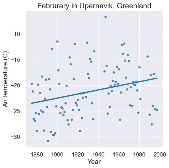
plot = feb.scatter('Year', 'Air temperature (C)', fit_line=True)
plot.set_title('Februrary in Upernavik, Greenland')
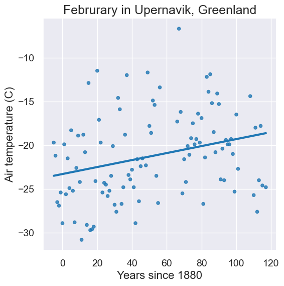
Let’s change the x-axis to be Years since 1880 so that it’s easier to calculate slope.
x = feb.column('Year') - 1880
y = feb.column('Air temperature (C)')
x_y_table = Table().with_columns("x", x, "y", y)
plot = x_y_table.scatter("x", "y", fit_line=True)
plot.set_xlabel("Years since 1880")
plot.set_ylabel("Air temperature (C)");
plot.set_title('Februrary in Upernavik, Greenland');
# Manually put in a, b
rise = -19+24
run = 120
a = rise/run
b = -24
print("a=", a, " , b=", b)
a= 0.041666666666666664 , b= -24
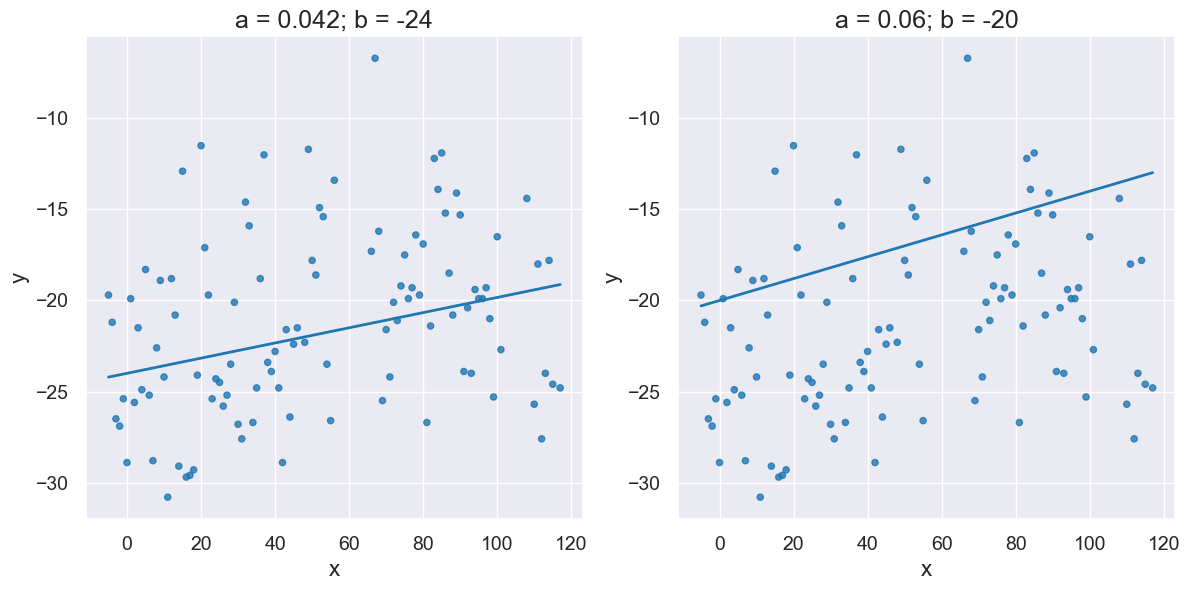
Two lines with different slopes and intercepts:
with Figure(1,2):
plot_scatter_with_line(x_y_table, 'x', 'y', a, b)
plot_scatter_with_line(x_y_table, 'x', 'y', 0.06, -20)
interact(plot_scatter_with_line,
table = Fixed(x_y_table),
x_label = Fixed('x'),
y_label = Fixed('y'),
a = Slider(-1,1,0.2),
b = Slider(-35,-8,2))
Here is an animation showing lines of different slope and intercept.
2. Predict and evaluate#
def line_predictions(a, b, x):
"""
Computes the prediction y_hat = a * x + b
where a and b are the slope and intercept and x is the set of x-values.
"""
return a * x + b
y_hat = line_predictions(a, b, x_y_table.column("x"))
prediction_table = x_y_table.with_columns("y_hat", y_hat)
prediction_table.take(np.arange(10, 15))
| x | y | y_hat |
|---|---|---|
| 5 | -18.3 | -23.7917 |
| 6 | -25.2 | -23.75 |
| 7 | -28.8 | -23.7083 |
| 8 | -22.6 | -23.6667 |
| 9 | -18.9 | -23.625 |
A “residual” is y - y_hat. In other words, a “residual” is the true y minus the prediction made by our line, y_hat.
residuals = prediction_table.column("y") - prediction_table.column("y_hat")
prediction_table = prediction_table.with_columns('residual', residuals)
prediction_table.show(3)
| x | y | y_hat | residual |
|---|---|---|---|
| -5 | -19.7 | -24.2083 | 4.50833 |
| -4 | -21.2 | -24.1667 | 2.96667 |
| -3 | -26.5 | -24.125 | -2.375 |
... (102 rows omitted)
interact(visualize_scatter_with_line_and_residuals,
table = Fixed(x_y_table),
x_label = Fixed('x'),
y_label = Fixed('y'),
a = Slider(-1,1,0.2),
b = Slider(-35,-8,2))
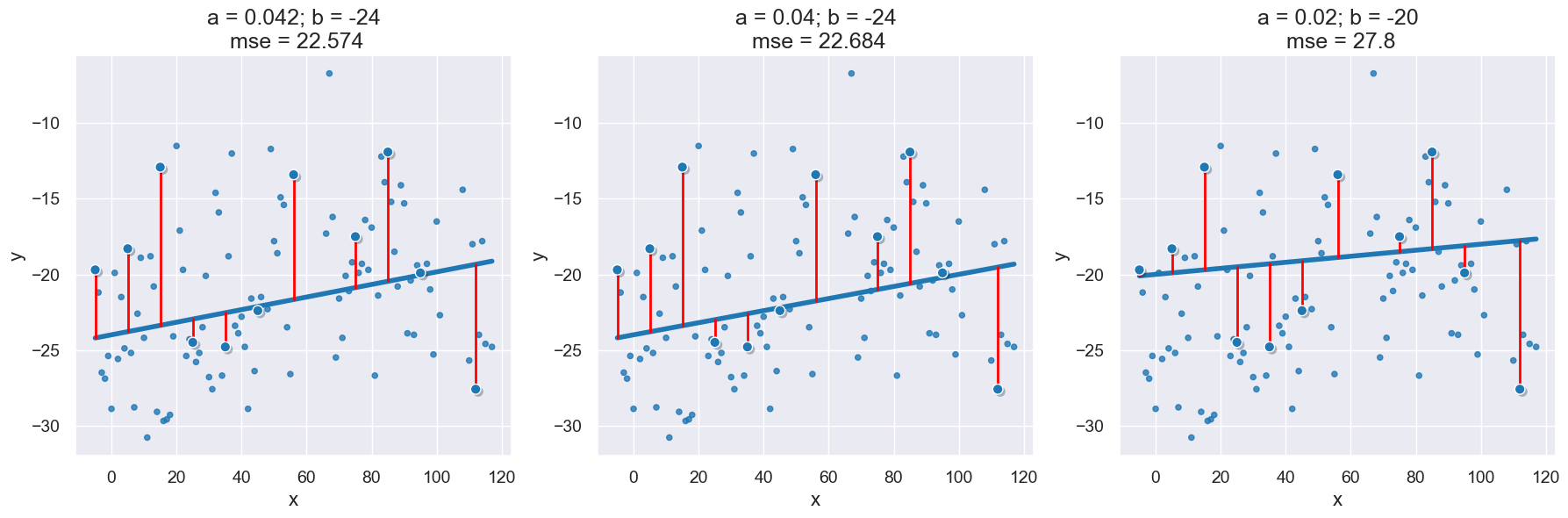
Here, mean squared error (MSE) first squares the residuals and then takes the mean.
Since we want our predictions (y_hat) to be closer to the observed values y a smaller MSE value is better.
np.mean(residuals**2)
22.57361111111111
Let’s write a function that computes the MSE for any table with data and line characterized by a and b.
def mean_squared_error(table, x_label, y_label, a, b):
y_hat = line_predictions(a, b, table.column(x_label))
residual = table.column(y_label) - y_hat
return np.mean(residual**2)
mean_squared_error(x_y_table, 'x', 'y', a, b)
22.57361111111111
mean_squared_error(x_y_table, 'x', 'y', 0.04, -24)
22.683558095238094
mean_squared_error(x_y_table, 'x', 'y', 0.02, -20)
27.799756190476195
interact(visualize_scatter_with_line_and_mse,
table = Fixed(x_y_table),
x_label = Fixed('x'),
y_label = Fixed('y'),
a = Slider(-1,1,0.2),
b = Slider(-35,-8,2))
with Figure(1,3):
visualize_scatter_with_line_and_mse(x_y_table, 'x', 'y', a, b)
visualize_scatter_with_line_and_mse(x_y_table, 'x', 'y', 0.04, -24)
visualize_scatter_with_line_and_mse(x_y_table, 'x', 'y', 0.02, -20)
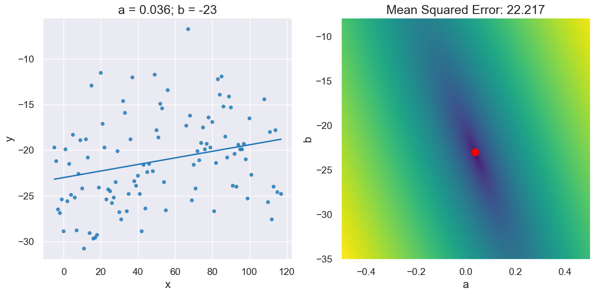
3. Fit the Best Line Manually#
visualize_regression_line_and_mse_heat(x_y_table, 'x', 'y')
Here is an animation showing how to manually fit a line using MSE.
4. Fit the Best Line with Brute Force#
# Brute force loop to find a and b
lowest_mse = np.inf
a_for_lowest = 0
b_for_lowest = 0
for a in np.arange(-0.5, 0.5, 0.001):
for b in np.arange(-35, -10, 1):
mse = mean_squared_error(x_y_table, 'x', 'y', a, b)
if mse < lowest_mse:
lowest_mse = mse
a_for_lowest = a
b_for_lowest = b
lowest_mse, a_for_lowest, b_for_lowest
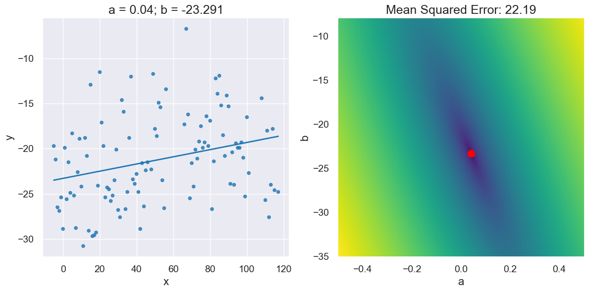
(22.216645485714288, 0.036000000000000476, -23)
# Looks pretty good when we plot it!
plot_regression_line_and_mse_heat(x_y_table, 'x', 'y', a_for_lowest, b_for_lowest)
5. Fit the Best Line with minimize()#
This is really an optimization problem for a curve in 3d.
plot_regression_line_and_mse_heat(x_y_table,
'x', 'y',
a_for_lowest, b_for_lowest,
show_mse='3d')
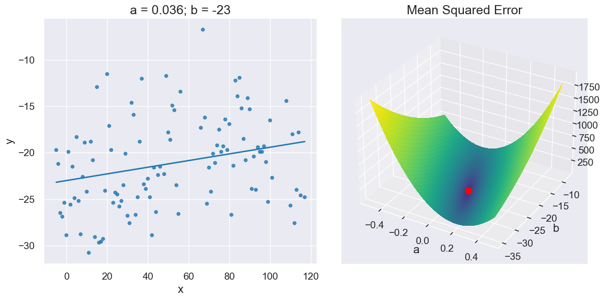
visualize_regression_line_and_mse_heat(x_y_table, 'x', 'y', show_mse='3d')
def linear_regression(table, x_label, y_label):
"""
Return an array containing the slope and intercept of the line best fitting
the table's data according to the mean square error loss function.
"""
# A helper function that takes *only* the two variables we need to optimize.
# This is necessary to use minimize below, because the function we want
# to minimize cannot take any parameters beyond those it will solve for.
def mse_for_a_b(a, b):
return mean_squared_error(table, x_label, y_label, a, b)
# We can use a built-in function minimize that uses gradient descent
# to find the optimal a and b for our mean squared error function
return minimize(mse_for_a_b)
optimal = linear_regression(x_y_table, 'x', 'y')
a_optimal = optimal.item(0)
b_optimal = optimal.item(1)
plot_regression_line_and_mse_heat(x_y_table, 'x', 'y', a_optimal, b_optimal)