Confidence Intervals

from datascience import *
from cs104 import *
import numpy as np
%matplotlib inline

1. Pea plants

Population: all 2nd generation plants

Sample: Mendel’s garden: 929 plants, 709 which had purple flowers

Statistic: Percent Purple

Load Data

mendel_garden = Table().read_table('data/mendel_garden_sample.csv')
mendel_garden.show(4)

Plant Number	Color
0	Purple
1	Purple
2	White
3	White

... (925 rows omitted)

mendel_garden.num_rows

929

color_array = mendel_garden.column("Color")

Our statistic is the percent purple.

def percent_purple(color): 
    proportion = sum(color == "Purple") / len(color)
    return proportion * 100 

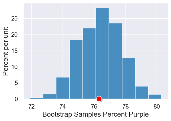
observed_stat = percent_purple(color_array)
observed_stat

76.31862217438106

Bootstrapping

Now we’re ready for our bootstrap_statistic function from our inference library.

results = bootstrap_statistic(color_array, percent_purple, 1000)

table = Table().with_columns("Bootstrap Samples Percent Purple", results)
plot = table.hist("Bootstrap Samples Percent Purple")
plot.dot(observed_stat)

2. Confidence Intervals

Percentiles

tiny_purple_stat = make_array(78, 70, 88, 82)
tiny_purple_stat

array([78, 70, 88, 82])

percentile(50, tiny_purple_stat)

78

percentile(75, tiny_purple_stat)

82

Confidence Intervals for Pea Plants

ci_percent = 95

percent_in_each_tail = (100 - ci_percent) / 2
percent_in_each_tail

2.5

left_end = percentile(percent_in_each_tail, results)
left_end

73.73519913885899

right_end = percentile(100 - percent_in_each_tail, results)
right_end

78.90204520990312

This function, which is also in our inference library, computes the desired confidence interval for an array of statistics.

def confidence_interval(ci_percent, statistics):
    """
    Return an array with the lower and upper bound of the ci_percent confidence interval.
    """
    # percent in each of the the left/right tails
    percent_in_each_tail = (100 - ci_percent) / 2   
    left = percentile(percent_in_each_tail, statistics)
    right = percentile(100 - percent_in_each_tail, statistics)
    return make_array(left, right)

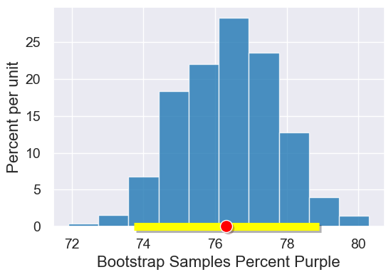
ci_95 = confidence_interval(95, results)
ci_95

array([73.73519914, 78.90204521])

table = Table().with_columns("Bootstrap Samples Percent Purple", results)
plot = table.hist("Bootstrap Samples Percent Purple")
plot.interval(ci_95)
plot.dot(observed_stat)

Different Confidence Intervals

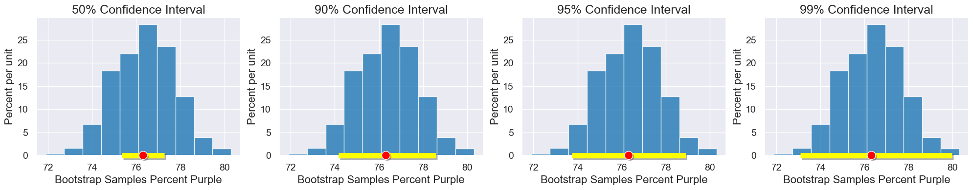
We can use confidence levels other than 95% too! Here is how the level impacts the size of the interval.

Our starting point:

confidence_interval(95, results)

array([73.73519914, 78.90204521])

If we’re okay with less confidence:

confidence_interval(90, results)

array([74.16576964, 78.57911733])

If we want more confidence:

confidence_interval(99, results)

array([73.08934338, 79.97847147])

We can see the impact of confidence level on the width of the interval more easily in the plots below.

def visualize_ci(ci_percent):
    """
    Plot the desired confidence interval for our Mendel bootstrap run above.
    """
    table = Table().with_columns("Bootstrap Samples Percent Purple", results)
    plot = table.hist("Bootstrap Samples Percent Purple")
    plot.set_title(str(ci_percent) + "% Confidence Interval")
    plot.interval(confidence_interval(ci_percent, results))
    plot.dot(observed_stat)    

with Figure(1,4, figsize=(5,4)):
    visualize_ci(50)
    visualize_ci(90)
    visualize_ci(95)
    visualize_ci(99)    

interact(visualize_ci, ci_percent=Slider(0,100,1))

ci_percent

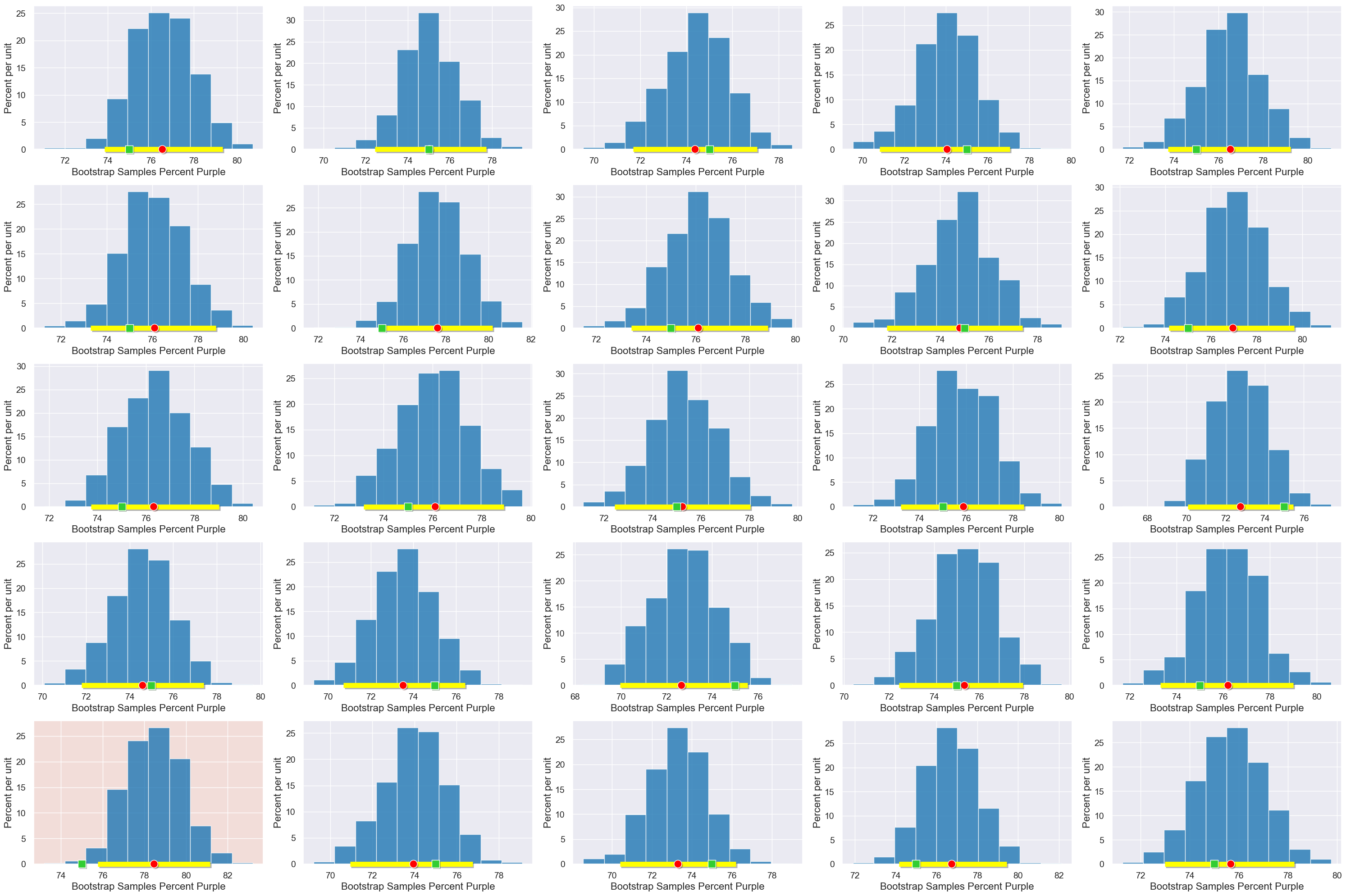
Interpreting Confidence

Here are 25 runs of our process on random samples. We expect 95% of our runs to produce confidence intervals containing the true parameter (75%).