Boostrapping
Contents
Boostrapping#
from datascience import *
from cs104 import *
import numpy as np
%matplotlib inline
1. Salary Data#
This is a dataset of salaries that came from a real-world survey. You can read more about this dataset here or here.
salaries = Table().read_table("data/salaries_clean.csv")
salaries = salaries.with_columns('Job title', salaries.apply(str.lower, 'Job title'))
salaries.show(5)
| Job title | Yearly Salary (USD) | Years Work Experience |
|---|---|---|
| research and instruction librarian | 55000 | 5-7 years |
| marketing specialist | 34000 | 2 - 4 years |
| program manager | 62000 | 8 - 10 years |
| accounting manager | 60000 | 8 - 10 years |
| scholarly publishing librarian | 62000 | 8 - 10 years |
... (23224 rows omitted)
data_jobs = salaries.where("Job title", are.containing("data"))
data_jobs.sample(5)
| Job title | Yearly Salary (USD) | Years Work Experience |
|---|---|---|
| data science manager | 220000 | 11 - 20 years |
| data scientist | 185000 | 5-7 years |
| data engineer | 89000 | 11 - 20 years |
| data scientist | 150000 | 5-7 years |
| data scientist | 95000 | 11 - 20 years |
data_jobs.num_rows
506
data_job_salaries = data_jobs.column("Yearly Salary (USD)")
Mean and median salaries#
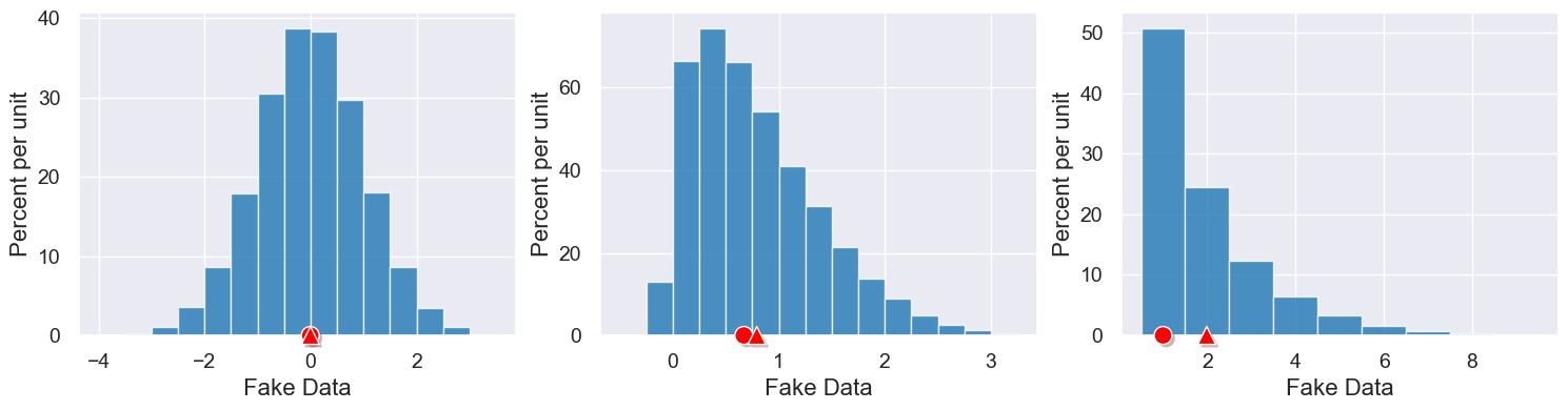
The mean is the “balancing point” of a histogram. The median is our “half-way point” of the data. For symmetric distributions, there are very close, but as a distribution becomes skewed to either larger or smaller values, they can become quite different:
Let’s explore the mean and median salaries for data jobs.
data_salary_mean = np.mean(data_job_salaries)
data_salary_mean
99742.75494071146
data_salary_median = np.median(data_job_salaries)
data_salary_median
92000.0
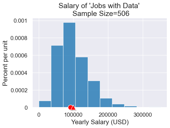
Here’s the mean (triangle) and median (circle) for our ‘Jobs with Data’ sample.
plot = data_jobs.hist("Yearly Salary (USD)")
plot.set_title("Salary of 'Jobs with Data' \n Sample Size="+str(data_jobs.num_rows))
plot.dot(data_salary_median)
plot.dot(data_salary_mean, marker='^')
2. Bootstrapping#
Given our sample, can we estimate the median salary for data jobs for the entire population?
Let’s sample with replacement for one sample.
print("Size of original sample", len(data_job_salaries))
Size of original sample 506
simulated_resample = np.random.choice(data_job_salaries, len(data_job_salaries))
print("Size after we resampled the original sample=", len(simulated_resample))
Size after we resampled the original sample= 506
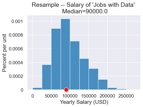
# Run many times
simulated_resample = np.random.choice(data_job_salaries, len(data_job_salaries))
median = np.median(simulated_resample)

table = Table().with_columns("Yearly Salary (USD)", simulated_resample)
plot = table.hist("Yearly Salary (USD)", bins=np.arange(0,300000,25000))
plot.set_title("Resample -- Salary of 'Jobs with Data' \n Median="+str(median))
plot.dot(median)
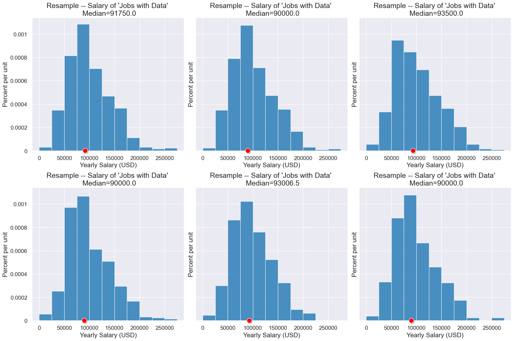
Here are some more resamples.
Let’s build a new simulation function to compute a statistic for many resamples. We’ll write it here, and it’s in our library for you to use.
def bootstrap_statistic(sample, compute_statistic, num_trials):
    """
    Creates num_trials resamples of the initial sample.
    Returns an array of the provided statistic for those samples.

    * sample: the initial sample, as an array.

    * compute_statistic: a function that takes a sample as
                         an array and returns the statistic for that
                         sample.

    * num_trials: the number of bootstrap samples to create.

    """
    statistics = make_array()

    for i in np.arange(0, num_trials):
        #Key: in bootstrapping we must always sample with replacement
        simulated_resample = np.random.choice(sample, len(sample))

        resample_statistic = compute_statistic(simulated_resample)
        statistics = np.append(statistics, resample_statistic)

    return statistics
results = bootstrap_statistic(data_job_salaries, np.median, 1000)
table = Table().with_columns("Yearly Salary (USD)", results)
plot = table.hist("Yearly Salary (USD)", bins=np.arange(87000,100000,1000))
plot.set_title("Bootstrap 1000 Times \n Sample Size="+str(data_jobs.num_rows))
plot.dot(data_salary_median)
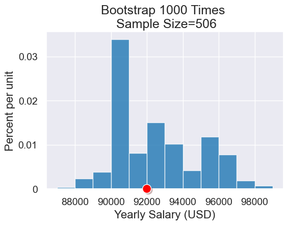
The above histogram captures the variability we see in the median salary in our resamples. That variability matches the variability we’d see in repeatedly sampling the whole population. We’ll see in the next lecture how to quantify the variability when estimating the median salary for the whole the population.