Randomized Controlled Experiments
Contents
Randomized Controlled Experiments#
from datascience import *
from cs104 import *
import numpy as np
%matplotlib inline
1. Warm-up Permutation Test#
survey = Table().read_table('data/prelab01-survey-fall2025.csv')
survey = survey.relabeled('Left or right handed? ', 'Left or Right Handed')  # clean up label
survey = survey.where('Left or Right Handed', are.not_equal_to('Ambidextrous'))
survey
| Favorite icecream flavor | Favorite planet | Height (in inches) | Distance Home (in miles) | Birthday month | Left or Right Handed |
|---|---|---|---|---|---|
| Mint chocolate chip | Neptune | 67 | 49 | September | Right handed |
| Vanilla | Neptune | 72 | 178 | December | Right handed |
| Purple Cow | Earth | 72 | 3058.6 | April | Right handed |
| Strawberry | Earth | 62 | 66 | July | Right handed |
| Strawberry | Earth | 66.5 | 185 | June | Left handed |
| Mint chocolate chip | Saturn | 65 | 2851.8 | January | Right handed |
| Purple Cow | Mars | 64 | 162 | February | Right handed |
| Mint chocolate chip | Earth | 68.5 | 120 | April | Right handed |
| Mint chocolate chip | Earth | 66 | 18.4 | January | Right handed |
| Chocolate | Earth | 68 | 146 | January | Right handed |
... (48 rows omitted)
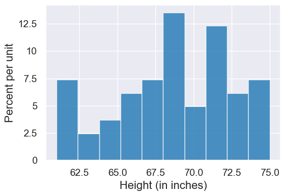
survey.hist('Height (in inches)')
survey.group('Left or Right Handed')
| Left or Right Handed | count |
|---|---|
| Left handed | 8 |
| Right handed | 50 |
observed = abs_difference_of_means(survey, 'Left or Right Handed', 'Height (in inches)')
observed
0.20049999999999102
Is the height difference significant?
results = simulate_permutation_statistic(survey, 'Left or Right Handed', 'Height (in inches)', 5000)
plot = Table().with_columns('abs_difference_of_means', results).hist(left_end=observed)
plot.set_title('Null hypothesis empirical distibution')
plot.dot(observed)
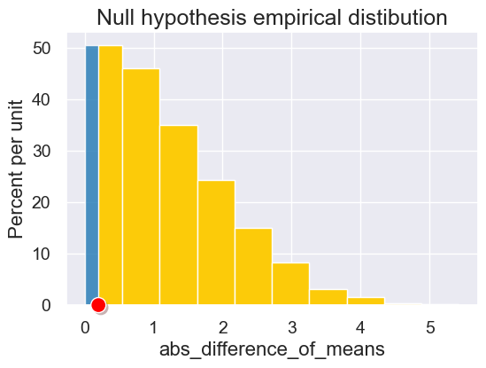
p_value = empirical_pvalue(results, observed)
p_value
0.9004
2. Randomized Controlled Experiment with BTA#
rct = Table.read_table('data/bta.csv')
rct.sample(10)
| Group | Result |
|---|---|
| Control | 0 |
| Control | 0 |
| Control | 0 |
| Control | 1 |
| Treatment | 1 |
| Treatment | 0 |
| Control | 0 |
| Control | 0 |
| Control | 0 |
| Control | 0 |
rct.group('Group')
| Group | count |
|---|---|
| Control | 16 |
| Treatment | 15 |
rct.pivot('Result', 'Group')
| Group | 0.0 | 1.0 |
|---|---|---|
| Control | 14 | 2 |
| Treatment | 6 | 9 |
rct.group('Group', np.mean)
| Group | Result mean |
|---|---|
| Control | 0.125 |
| Treatment | 0.6 |
Permutation Testing#
observed_statistic = abs_difference_of_means(rct, 'Group', 'Result')
observed_statistic
0.475
type(observed_statistic)
float
results = simulate_permutation_statistic(rct, 'Group', 'Result', 2000)
plot = Table().with_columns('Abs Difference in Relief Proportions', results).hist(bins=np.arange(0,0.9,1/16))
plot.set_title('Null hypothesis empirical distibution')
plot.dot(observed_statistic)
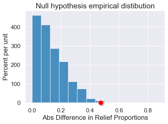
p_value = empirical_pvalue(results, observed_statistic)
p_value
0.0095
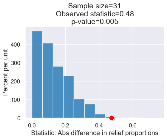
3. Sample Size, Effect Size, and P-values#
What’s the relationship between effect size, sample size, and p-value?
What we had before.
What if the effect size was slightly smaller? What if the sample size was bigger?
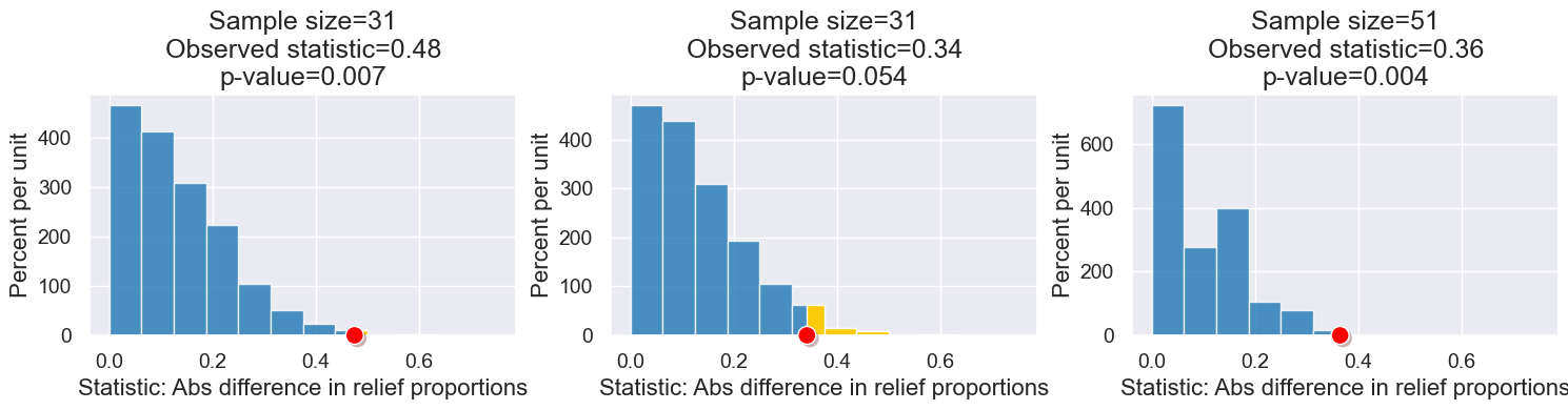
Let’s look at all these relationships at once!
interact(back_pain_exploration,
         observed_sample_size=Slider(10, 128, 1),
         treatment_prop_effective=Slider(0.05, 0.95, 0.01),
         control_prop_effective=Slider(0.05, 0.95, 0.01))
Here’s an animation showing the effects above.