Assessing Models

from datascience import *
from cs104 import *
import numpy as np
%matplotlib inline

1. Mendel and Pea Flowers

We know we’ll be using our simulate_sample_statistic from our inference library, so let’s build and check all these pieces!

simulate_sample_statistic(
   make_one_sample,
   sample_size,
   compute_sample_statistic,
   num_trials)

Observed sample: In Mendel’s one sample (his own garden), he had 929 second new generation pea plants, of which 709 had purple flowers. We compute the percent purple he observed:

observed_sample_size = 929
observed_purple_percent = 709 / observed_sample_size * 100
observed_purple_percent

76.31862217438106

Model: Mendel hypothesized (based on his preliminary theories of genetics) that he should have gotten 75% purple and 25% white.

hypothesized_purple_proportion = 0.75

Let’s represent our population as an array showing the proportion of purple and white flowers under our model assumption. (This sets us up for sampling…)

hypothesized_proportions = make_array(hypothesized_purple_proportion, 
                                      1 - hypothesized_purple_proportion) 
hypothesized_proportions

array([0.75, 0.25])

In the Python library reference, we see can use the function sample_proportions(sample_size, model_proportions) to sample based on those proportions. We want to represent our sample as the percent purple and percent white, so don’t forget to multiply by 100!

sample = 100 * sample_proportions(observed_sample_size, hypothesized_proportions)
sample

array([76.74919268, 23.25080732])

Let’s put it into a function.

def flowers_make_sample(sample_size): 
    """
    Return the percents of purple flowers and white flowers in an array
    """
    hypothesized_purple_proportion = 0.75
    hypothesized_proportions = make_array(hypothesized_purple_proportion, 
                                          1 - hypothesized_purple_proportion) 
    sample = 100 * sample_proportions(sample_size, hypothesized_proportions)
    return sample

flowers_make_sample(10)

array([70., 30.])

flowers_make_sample(observed_sample_size)

array([77.71797632, 22.28202368])

The two items in the array returned from our sampling function correspond to the percent of purple and white flowering plants in our sample. So the “percent purple” statistic is defined as follows:

def stat_percent_purple(sample): 
    return sample.item(0)

stat_percent_purple(sample)

76.7491926803014

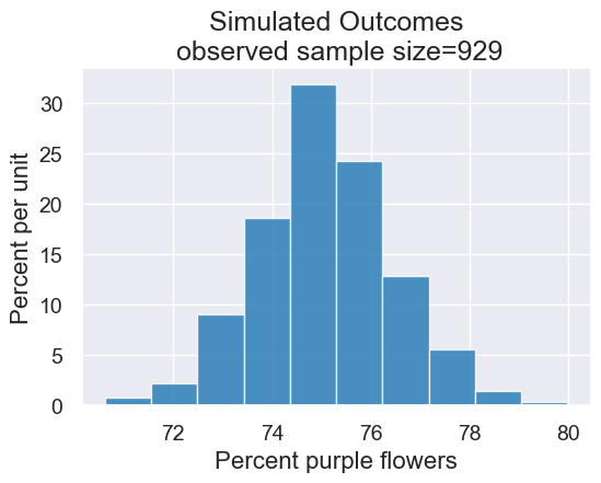
Now let’s use our function simulate_sample_statistic.

num_trials = 1000

all_outcomes = simulate_sample_statistic(flowers_make_sample, observed_sample_size,
                                         stat_percent_purple, num_trials)

results = Table().with_column('Percent purple flowers', all_outcomes)
plot = results.hist()
plot.set_title('Simulated Outcomes\n observed sample size=' + str(observed_sample_size))

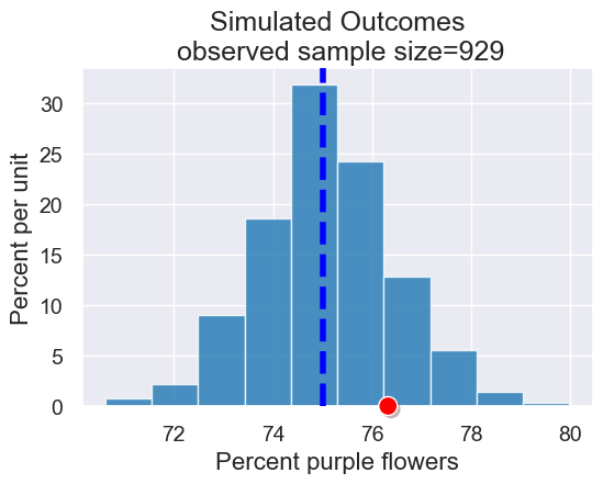
Connecting these pieces together:

• In Mendel’s model, he hypothesized getting purple flowers was like flipping a biased coin and getting heads 75% of the time.

• We simulated outcomes under this hypothesis.

• Now let’s check if the observed data (that there were 76.3% purple flowers in one sample, Mendel’s own garden) “fits” with the simulated outcomes under the model

plot = results.hist()
plot.set_title('Simulated Outcomes\n observed sample size=' + str(observed_sample_size))
plot.line(x=75,lw=4,linestyle="dashed")
plot.dot(observed_purple_percent)

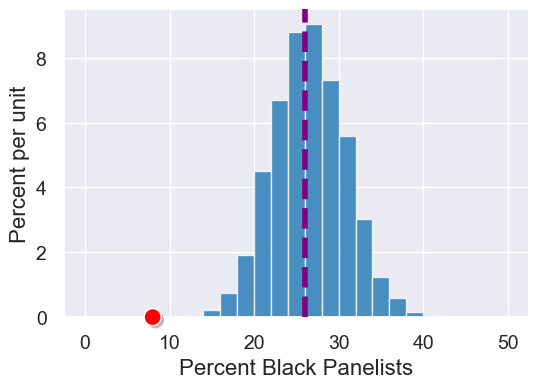
2. Swain vs. Alabama

In the 1960s, eligible juror population at the time was men who were at 21 years old.

In Talladega County, where the trial was held, 26% of the eligible jurors were Black. The 100-person panel of prospective jurors had 8 Black individuals. Should we expect this situation to happen frequently? Sometimes? Ever?

Once again, we’ll be using our algorithm/function for simulating statistics.

simulate_sample_statistic(make_sample,
   sample_size,
   compute_statistic,
   num_trials)

Make one sample. We will sample panels from our hypothesized categorical distribution (26% Black and 74% non-Black jurors) which is the same oas the eligible juror population.

population_percent_black = 26
population_proportions = make_array(population_percent_black / 100,
                                    1 - population_percent_black / 100)
population_proportions

array([0.26, 0.74])

sample_size = 10
sample_proportions(sample_size, population_proportions)

array([0.5, 0.5])

def simulate_panel_selection(sample_size):
    """Return an array with the counts of [black, non-black] panelists in sample."""
    props = sample_proportions(sample_size, population_proportions)
    return np.round(sample_size * props)  # no fractional persons

sample = simulate_panel_selection(100)
sample 

array([22., 78.])

def percent_black_statistic(sample): 
    """ Percent black panelists (for any sample size)"""
    return sample.item(0) / sum(sample) * 100

percent_black_statistic(sample)

22.0

Now we’re ready to use simulate_sample_statistic.

sample_size = 100 # The actual observed number of panelists
num_trials = 5000
all_outcomes = simulate_sample_statistic(simulate_panel_selection, sample_size, 
                                         percent_black_statistic, num_trials)

Let’s plot to create the empirical distribution with our hypothesis.

simulated_black_panelists_results = Table().with_column('Percent Black Panelists', 
                                                        all_outcomes)
plot = simulated_black_panelists_results.hist(bins=np.arange(0, 51, 2))

# Purple line for the model parameter
plot.line(x = population_percent_black, linestyle="--", color='purple', width=4)

# Red dot for the statistic on the observed (not simulated) data
observed_black_panelists_count = 8
plot.dot(observed_black_panelists_count)