Inference with Statistics
Contents
Inference with Statistics#
from datascience import *
from cs104 import *
import numpy as np
%matplotlib inline
1. Snoopy’s Fleet#
We will create a simulation for the empirical distribution of our chosen statistic.
At true inference time, we do not know N. However, let’s create N now so that we can evaluate how “good” our chosen models and statistics could be.
N = 300
population = np.arange(1, N+1)
Suppose we didn’t know N. Then all we could do is observe samples of planes flying overhead.
We’ll use our model assumption: Plane numbers are uniform random sample drawn with replacement from 1 to N.
def sample_plane_fleet(sample_size):
    return np.random.choice(population, sample_size)
sample = sample_plane_fleet(10)
sample
array([155, 3, 123, 123, 232, 60, 13, 230, 231, 109])
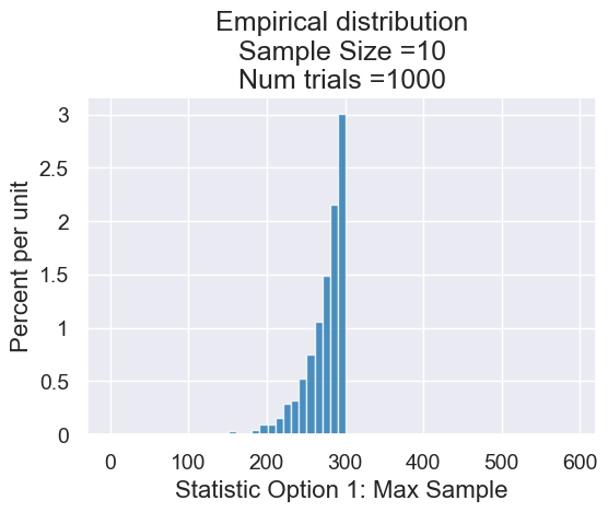
Option 1: Sample Statistic is the max plane number#
Let’s choose a stastic as the max of as sample. Luckily, max is simple and we don’t have to write a new function here. We can use Python’s built-in function!
max(sample)
232
Let’s put this all together using our simulation algorithm.
sample_size = 10
num_trials = 1000
all_outcomes = simulate_sample_statistic(sample_plane_fleet, sample_size,
                                         max, num_trials)

results = Table().with_columns("Statistic Option 1: Max Sample", all_outcomes)
plot = results.hist(bins=np.arange(1, 2 * N, 10))
plot.set_title("Empirical distribution\n"+
               "Sample Size ="+str(sample_size)+
               "\nNum trials ="+str(num_trials))
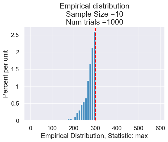
Let’s generalize a bit and create function that takes the statistic and runs the whole experiment.
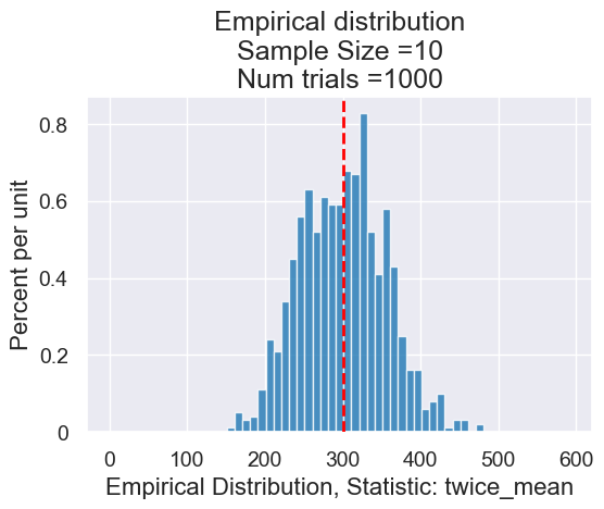
Option 2: Sample Statistic is Twice the Mean#
Let’s generalize a bit and create function that takes the statistic and runs the whole experiment
def planes_empirical_statistic_distribution(sample_size, compute_sample_statistic, num_trials):
    """
    Simulates multiple trials of a statistic on our simulated fleet of N planes

    Inputs
        - sample_size: number of planes we see in our sample
        - compute_sample_statistic: a function that takes an array
            and returns a summary statistic (e.g. max)
        - num_trials: number of simulation trials

    Output
        Histogram of the results
    """
    all_outcomes = simulate_sample_statistic(sample_plane_fleet, sample_size,
                                             compute_sample_statistic, num_trials)

    results = Table().with_columns('Empirical Distribution, Statistic: ' + compute_sample_statistic.__name__,
                                   all_outcomes)
    plot = results.hist(bins=np.arange(1, 2 * N, 10))
    plot.set_title("Empirical distribution\n"+
               "Sample Size ="+str(sample_size)+
               "\nNum trials ="+str(num_trials))

    # Red line is the True N
    plot.line(x=N, color='r', linestyle='--')
planes_empirical_statistic_distribution(10, max, 1000)
Our second option for the statistic:
def twice_mean(sample):
    """Twice the sample mean"""
    return 2 * np.mean(sample)

planes_empirical_statistic_distribution(10, twice_mean, 1000)
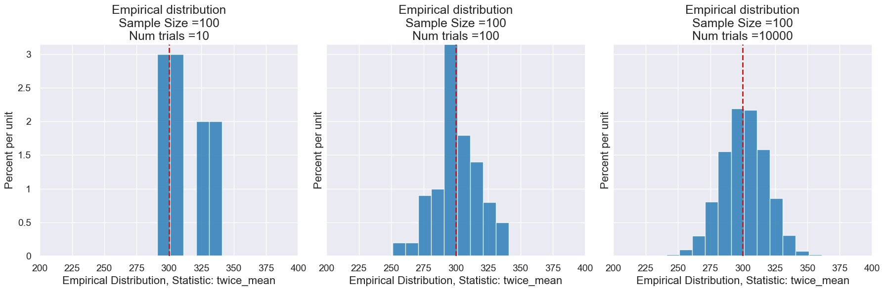
2.Effects of Sample Size and Simulation Rounds#
First interaction: Let’s just look at the number of trials just for our twice mean statistic with everything else held constant.
interact(planes_empirical_statistic_distribution,
         sample_size=Fixed(20),
         compute_sample_statistic=Fixed(twice_mean),
         num_trials=Slider(1, 20010, 10))
Here are a few sample distrubtions with different numbers of trials.
We can also examinge the impact of changing the sample size and N using the following function.
def visualize_distributions(N, sample_size, num_trials):
    """A single function to run our simulation for a given N, sample_size, and num_trials."""
    import matplotlib.pyplot as plt

    population = np.arange(1, N+1)

    # Builds up our outcomes table one row at a time.  We do this to ensure
    # we can apply both statistics to the same samples.
    outcomes_table = Table(["Max", "2*Mean"])

    for i in np.arange(num_trials):
        sample = np.random.choice(population, sample_size)
        outcomes_table.append(make_array(max(sample), 2 * np.mean(sample)))

    plot = outcomes_table.hist(bins=np.arange(N/2, 3*N/2, 2))
    plot.set_title("Empirical distribution (N="+str(N)+")\n"+
               "Sample size ="+str(sample_size)+
               "\nNum trials ="+str(num_trials))
    # Red line is the True N
    plot.line(x=N, color='r', linestyle='--')
interact(visualize_distributions,
         N=Slider(100, 450, 50),
         sample_size=Slider(10, 101, 1),
         num_trials=Slider(10, 10100, 100))
Here’s a visualization of how sample size impacts the distribution of our statistic for random samples.
Here’s a visualization of how the number of trials impacts the distribution of our statistic for random samples.
Here’s a visualization of how the parameter N impacts the distribution of our statistic for random samples.
3. Mendel and Pea Flowers#
Looking ahead, we know we’ll be using our simulate sample statistc! So let’s build and check all these pieces.
simulate_sample_statistic(make_sample,
   sample_size,
   compute_statistic,
   num_trials)
Observed sample: In Mendel’s one sample (his own garden), he had 929 second new generation pea plants, of which 709 had purple flowers. We compute the percent purple he observed:
observed_sample_size = 929
observed_purples = 709 / observed_sample_size * 100
observed_purples
76.31862217438106
Model: Mendel hypothesized (based on his preliminary theories of genetics) that he should have gotten 75% purple and 25% white.
hypothesized_purple_proportion = 0.75
hypothesized_proportions = make_array(hypothesized_purple_proportion,
                                      1 - hypothesized_purple_proportion)
hypothesized_proportions
array([0.75, 0.25])
In the Python library reference, we see can use the function sample_proportions(sample_size, model_proportions).
sample = sample_proportions(observed_sample_size, hypothesized_proportions)
sample
array([0.7664155, 0.2335845])
Let’s put it into a function.
def flowers_make_sample(sample_size):
    """
    Return the percents of purple flowers and white flowers in an array
    """
    hypothesized_purple_proportion = 0.75
    hypothesized_proportions = make_array(hypothesized_purple_proportion,
                                          1 - hypothesized_purple_proportion)
    sample = 100 * sample_proportions(sample_size, hypothesized_proportions)
    return sample
flowers_make_sample(observed_sample_size)
array([75.67276642, 24.32723358])
Each item in the array corresponds to the proportion of times it was sampled out of sample_size times. So the proportion purple is
def stat_percent_purple(sample):
    return sample.item(0)

stat_percent_purple(sample)
0.7664155005382132
Now let’s use our function simulate_sample_statistic.
num_trials = 1000

all_outcomes = simulate_sample_statistic(flowers_make_sample, observed_sample_size,
                                         stat_percent_purple, num_trials)
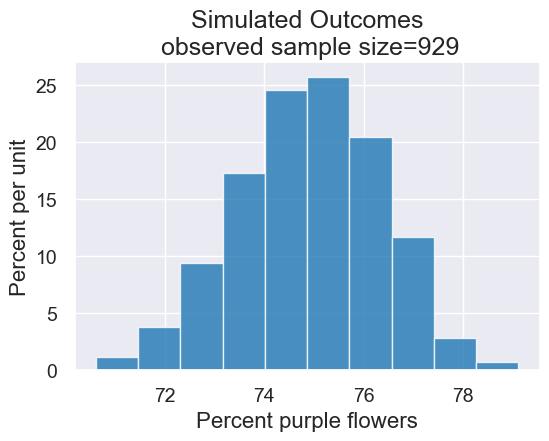
results = Table().with_column('Percent purple flowers', all_outcomes)
results.hist(title = 'Simulated Outcomes\n observed sample size=' + str(observed_sample_size))
Connecting these pieces together:
In Mendel’s model, he hypothesized getting purple flowers was like flipping a biased coin and getting heads 75% of the time.
We simulated outcomes under this hypothesis.
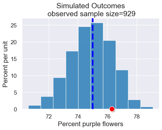
Now let’s check if the observed data (that there were 76.3% purple flowers in one sample, Mendel’s own garden) “fits” with the simulated outcomes under the model
plot = results.hist(title = 'Simulated Outcomes\n observed sample size=' + str(observed_sample_size))
plot.line(x=75,lw=4,linestyle="dashed")
plot.dot(observed_purples)
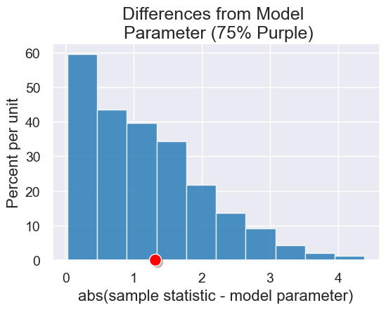
differences_from_model = Table().with_column('abs(sample statistic - model parameter)',
                                             abs(all_outcomes - 75))

diff_plot = differences_from_model.hist(title = 'Differences from Model \n Parameter (75% Purple)')
diff_plot.dot(abs(observed_purples - 75))
Once again, let’s use computation to abstract away the variables that we have the power to change, and the parts of the code that never change. Here is a new function to do that.
def pea_plants_simulation(observed_sample_size, observed_purples_count,
                          hypothesized_purple_percent, num_trials):
    """
    Parameters:
        - observed_sample_size: number of plants in our experiment
        - observed_purples_count: count of plants in our experiment w/ purple flowers
        - hypothesized_purple_proportion: our model parameter (hypothesis for
              proportion of plants will w/ purple flowers).
        - num_trials: number of simulation rounds to run
    Outputs two plots:
        - Empirical distribution of the percent of plants w/ purple flowers
          from our simulation trials
        - Empirical distribution of how far off each trial was from our hypothesized model
    """

    observed_purples = 100 * observed_purples_count / observed_sample_size
    hypothesized_proportions = make_array(hypothesized_purple_percent/100,
                                          1 - hypothesized_purple_percent/100)

    assert 0 <= hypothesized_proportions[0] <= 1, str(hypothesized_proportions)
    assert 0 <= hypothesized_proportions[1] <= 1, str(hypothesized_proportions)

    all_outcomes = make_array()
    for i in np.arange(0, num_trials):
        simulated_sample = 100 * sample_proportions(observed_sample_size, hypothesized_proportions)
        outcome = simulated_sample.item(0)
        all_outcomes = np.append(all_outcomes, outcome)

    #plots
    with Figure(1,2):
        percent_purple = Table().with_column('% of purple flowers', all_outcomes)
        pp_plot = percent_purple.hist(title='Simulated Outcomes\n observed sample size=' + str(observed_sample_size))
        pp_plot.dot(observed_purples)

        distance_from_model = Table().with_column('abs(sample statistic - model parameter)',
                                                  abs(all_outcomes - hypothesized_purple_percent))
        dist_plot = distance_from_model.hist(title='Differences from Model \n Parameter (' + str(hypothesized_purple_percent) + '% Purple)')
        dist_plot.dot(abs(observed_purples - hypothesized_purple_percent))
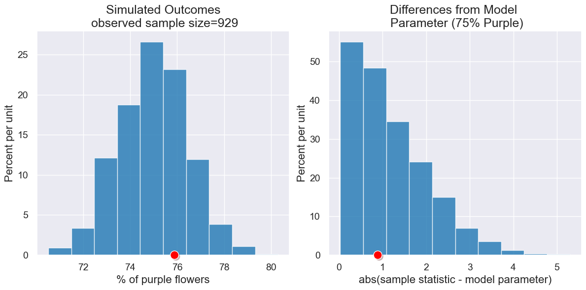
Here is a scenario to match Mendel’s garden. 705 out of 929 plants had purple flowers, and he proposed 75% should be purple.
pea_plants_simulation(929, 705, 75, 1000)
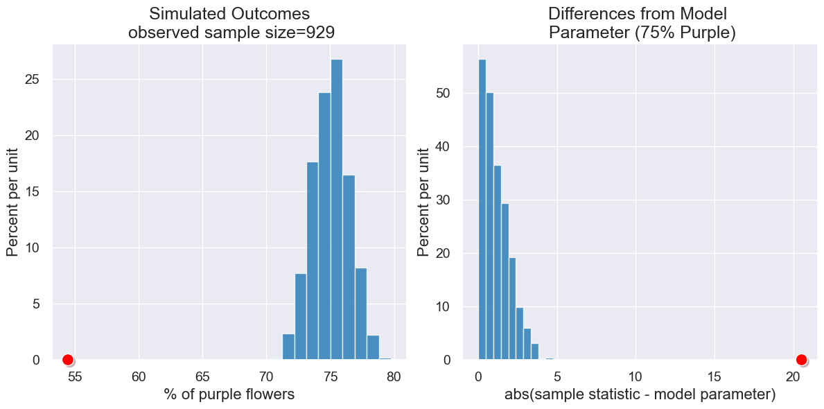
Here is a different scenario. Suppose only 506 out of 929 plants had purple flowers, and but our model indicates that 75% should be purple.
pea_plants_simulation(929, 506, 75, 1000)
interact(pea_plants_simulation,
         observed_sample_size = Fixed(929),
         observed_purples_count = Slider(0,929),
         hypothesized_purple_percent = Slider(0,100,1),
         num_trials=Slider(10, 5000, 100))