Probability and Sampling
Contents
Probability and Sampling#
from datascience import *
from cs104 import *
import numpy as np
%matplotlib inline
1. Distributions#
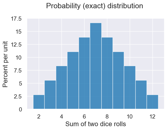
Probability Distribution#
We can use probability rules to analytically write down the expected number of each possible value in order to create a probability distribution like the following
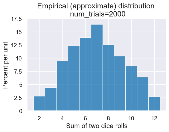
Empirical Distribution#
dice = np.arange(1,7)
dice
array([1, 2, 3, 4, 5, 6])
Let’s roll the dice twice and add the values.
two_dice = np.random.choice(dice, 2)
print('two dice=', two_dice)
print('sum=', sum(two_dice))
two dice= [6 1]
sum= 7
Let’s put this together in a function that simulate can use as an input.
def sum_two_dice():
    dice = np.arange(1,7)
    two_dice = np.random.choice(dice, 2)
    return sum(two_dice)
Use simulate (from our inference library) to create an empirical distribution.
def simulate(make_one_outcome, num_trials):
    """
    Return an array of num_trials values, each
    of which was created by calling make_one_outcome().
    """
    outcomes = make_array()
    for i in np.arange(0, num_trials):
        outcome = make_one_outcome()
        outcomes = np.append(outcomes, outcome)

    return outcomes
num_trials = 10
simulate(sum_two_dice, num_trials)
array([ 9., 7., 6., 5., 5., 7., 11., 2., 4., 3.])
num_trials = 2000
all_outcomes = simulate(sum_two_dice, num_trials)
simulated_results = Table().with_column('Sum of two dice rolls', all_outcomes)
simulated_results
| Sum of two dice rolls |
|---|
| 9 |
| 7 |
| 4 |
| 5 |
| 11 |
| 8 |
| 11 |
| 6 |
| 10 |
| 9 |
... (1990 rows omitted)
plot = simulated_results.hist(bins=outcome_bins)
plot.set_title('Empirical (approximate) distribution \n num_trials='+str(num_trials));
plot.set_ylim(0,0.175)
Law of Averages#
In our simulation, we have one parameter that we have the ability to control num_trials. Does this parameter matter?
To find out, we can write a function that takes as input the num_trials parameter.
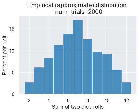
def simulate_and_plot_summing_two_dice(num_trials):
    """
    Simulates rollowing two dice and repeats num_trials times, and
    Plots the empirical distribution
    """
    all_outcomes = simulate(sum_two_dice, num_trials)
    simulated_results = Table().with_column('Sum of two dice rolls', all_outcomes)

    outcome_bins = np.arange(1.5, 13.5, 1)
    plot = simulated_results.hist(bins=outcome_bins)
    plot.set_title('Empirical (approximate) distribution \n num_trials='+str(num_trials))
    plot.set_ylim(0,0.18)
simulate_and_plot_summing_two_dice(2000)
Here are a couple plots for different numbers of trials:
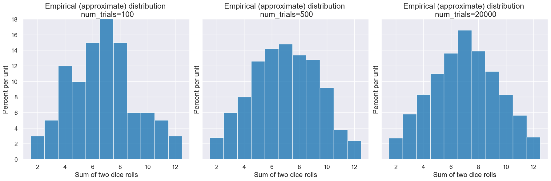
interact(simulate_and_plot_summing_two_dice, num_trials = Slider(1,1000))
Here is an animation also showing how the number of trials impacts the result for a wider range of values.
2. Random Sampling: Florida Votes in 2016#
Load data for voting in Florida in 2016. These give us the true parameters if we were able to poll every person who would turn out to vote:
Proportion voting for (Trump, Clinton, Johnson, other) = (0.49, 0.478, 0.022, 0.01)
Raw counts:
Trump: 4,617,886
Clinton: 4,504,975
Johnson: 207,043
Other: 90,135
Data is based on the actual votes case in the election.
votes = Table().read_table('data/florida_2016.csv')
votes = votes.with_column('Vote', votes.apply(make_array("Trump", "Clinton", "Johnson", "Other").item, "Vote"))
votes.show(5)
| Vote |
|---|
| Clinton |
| Trump |
| Trump |
| Clinton |
| Trump |
... (9420034 rows omitted)
Here’s the total number of votes cast in the election.
votes.num_rows
9420039
We can pick a “convenience sample”: the first 10 voters who show up in line.
votes.take(np.arange(10))
| Vote |
|---|
| Clinton |
| Trump |
| Trump |
| Clinton |
| Trump |
| Johnson |
| Clinton |
| Clinton |
| Clinton |
| Trump |
Since we are analyzing this after the election, we actually know the votes for the full population and we can compute the true parameter.
sum(votes.column('Vote') == 'Trump') / votes.num_rows
0.49021941416590736
But suppose this is before the election and we actually can’t ask every person in the state how they will vote…
In that case, we can imagine we are a pollster, and sample 50 people.
We can use .sample(n) to randomly sample n rows from a table.
sample = votes.sample(50)
sample
| Vote |
|---|
| Trump |
| Clinton |
| Clinton |
| Trump |
| Trump |
| Clinton |
| Clinton |
| Trump |
| Clinton |
| Clinton |
... (40 rows omitted)
sum(sample.column('Vote') == 'Trump') / sample.num_rows
0.54
Let’s write functions to do this!
A function that takes a sample
A function that computes the statistic (proportion of the sample that voted for Trump).
def sample_votes(sample_size):
    return votes.sample(sample_size)
def proportion_vote_trump(sample):
    return sum(sample.column('Vote') == 'Trump') / sample.num_rows
sample = sample_votes(100)
proportion_vote_trump(sample)
0.51
proportion_vote_trump(sample_votes(100))
0.53
proportion_vote_trump(sample_votes(1000))
0.509
So far, we’ve been using a simulate function. Let’s extend this to a function that can also take a sample size. We’ll call this function simulate_sample_statistic.
def simulate_sample_statistic(make_one_sample, sample_size,
                              compute_sample_statistic, num_trials):
    """
    Simulates num_trials sampling steps and returns an array of the
    statistic for those samples.  The parameters are:

    - make_one_sample: a function that takes an integer n and returns a
                   sample as an array of n elements.

    - sample_size: the size of the samples to use in the simulation.

    - compute_statistic: a function that takes a sample as
                         an array and returns the statistic for that sample.

    - num_trials: the number of simulation steps to perform.
    """

    simulated_statistics = make_array()
    for i in np.arange(0, num_trials):
        simulated_sample = make_one_sample(sample_size)
        sample_statistic = compute_sample_statistic(simulated_sample)
        simulated_statistics = np.append(simulated_statistics, sample_statistic)
    return simulated_statistics
Let’s use our simulation algorithm to create an empirical distribution.
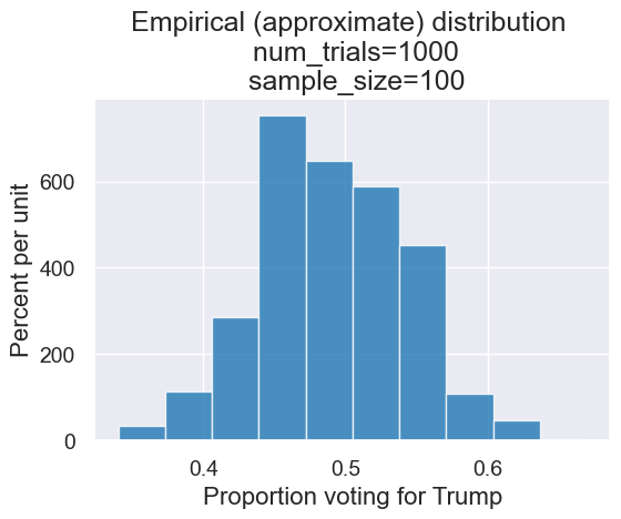
Suppose there are 1,000 polling companies and each uses a sample of 100 people.
num_trials = 1000 #1,000 polling companies
sample_size = 100 #100 people sampled by each polling company

all_outcomes = simulate_sample_statistic(sample_votes, sample_size,
                                         proportion_vote_trump, num_trials)
all_outcomes
array([0.5 , 0.57, 0.51, 0.48, 0.53, 0.54, 0.47, 0.47, 0.45, 0.56, 0.43,
       0.42, 0.53, 0.41, 0.54, 0.5 , 0.37, 0.54, 0.42, 0.49, 0.48, 0.47,
       0.45, 0.52, 0.46, 0.42, 0.51, 0.47, 0.52, 0.53, 0.54, 0.56, 0.39,
       0.55, 0.48, 0.49, 0.46, 0.45, 0.54, 0.54, 0.56, 0.4 , 0.59, 0.48,
       0.5 , 0.47, 0.47, 0.55, 0.52, 0.48, 0.55, 0.47, 0.44, 0.49, 0.44,
       0.47, 0.52, 0.59, 0.45, 0.53, 0.53, 0.51, 0.42, 0.46, 0.52, 0.48,
       0.42, 0.48, 0.52, 0.41, 0.5 , 0.47, 0.49, 0.43, 0.44, 0.51, 0.48,
       0.5 , 0.54, 0.51, 0.43, 0.41, 0.52, 0.48, 0.45, 0.47, 0.44, 0.53,
       0.46, 0.53, 0.41, 0.42, 0.4 , 0.47, 0.53, 0.6 , 0.48, 0.58, 0.45,
       0.39, 0.47, 0.47, 0.48, 0.41, 0.46, 0.5 , 0.55, 0.57, 0.54, 0.38,
       0.49, 0.53, 0.45, 0.48, 0.45, 0.56, 0.57, 0.35, 0.35, 0.59, 0.56,
       0.44, 0.44, 0.48, 0.53, 0.53, 0.51, 0.41, 0.34, 0.51, 0.51, 0.42,
       0.44, 0.46, 0.53, 0.56, 0.45, 0.44, 0.5 , 0.41, 0.44, 0.54, 0.54,
       0.44, 0.43, 0.44, 0.54, 0.42, 0.48, 0.58, 0.53, 0.48, 0.43, 0.47,
       0.55, 0.57, 0.48, 0.53, 0.51, 0.5 , 0.51, 0.51, 0.51, 0.49, 0.54,
       0.49, 0.47, 0.6 , 0.45, 0.56, 0.53, 0.49, 0.57, 0.46, 0.44, 0.59,
       0.42, 0.55, 0.48, 0.43, 0.44, 0.53, 0.51, 0.47, 0.39, 0.53, 0.55,
       0.47, 0.45, 0.51, 0.52, 0.47, 0.5 , 0.47, 0.53, 0.39, 0.5 , 0.49,
       0.49, 0.43, 0.49, 0.54, 0.54, 0.5 , 0.47, 0.52, 0.45, 0.6 , 0.54,
       0.48, 0.43, 0.4 , 0.49, 0.36, 0.63, 0.49, 0.48, 0.53, 0.49, 0.61,
       0.5 , 0.46, 0.38, 0.45, 0.5 , 0.43, 0.49, 0.45, 0.58, 0.51, 0.57,
       0.48, 0.42, 0.43, 0.52, 0.55, 0.53, 0.48, 0.45, 0.4 , 0.47, 0.49,
       0.46, 0.56, 0.43, 0.45, 0.43, 0.54, 0.52, 0.42, 0.55, 0.46, 0.49,
       0.47, 0.48, 0.51, 0.52, 0.46, 0.49, 0.48, 0.47, 0.52, 0.5 , 0.47,
       0.49, 0.57, 0.55, 0.47, 0.54, 0.5 , 0.63, 0.48, 0.47, 0.61, 0.49,
       0.5 , 0.48, 0.6 , 0.47, 0.45, 0.43, 0.42, 0.45, 0.51, 0.46, 0.47,
       0.47, 0.53, 0.57, 0.57, 0.49, 0.56, 0.48, 0.47, 0.58, 0.4 , 0.47,
       0.35, 0.46, 0.48, 0.51, 0.51, 0.58, 0.49, 0.52, 0.47, 0.46, 0.47,
       0.42, 0.49, 0.52, 0.54, 0.48, 0.46, 0.59, 0.51, 0.53, 0.44, 0.46,
       0.41, 0.49, 0.61, 0.43, 0.42, 0.51, 0.52, 0.51, 0.46, 0.52, 0.5 ,
       0.54, 0.57, 0.55, 0.43, 0.54, 0.47, 0.5 , 0.56, 0.55, 0.51, 0.49,
       0.42, 0.48, 0.53, 0.54, 0.44, 0.55, 0.5 , 0.45, 0.53, 0.56, 0.5 ,
       0.47, 0.5 , 0.5 , 0.5 , 0.45, 0.42, 0.55, 0.49, 0.47, 0.5 , 0.53,
       0.52, 0.51, 0.44, 0.47, 0.58, 0.53, 0.46, 0.43, 0.56, 0.45, 0.46,
       0.55, 0.55, 0.45, 0.44, 0.47, 0.44, 0.5 , 0.45, 0.51, 0.47, 0.49,
       0.45, 0.59, 0.34, 0.48, 0.55, 0.47, 0.54, 0.56, 0.56, 0.51, 0.5 ,
       0.53, 0.44, 0.48, 0.41, 0.52, 0.58, 0.54, 0.46, 0.48, 0.48, 0.4 ,
       0.45, 0.45, 0.44, 0.39, 0.47, 0.47, 0.59, 0.61, 0.42, 0.56, 0.55,
       0.48, 0.52, 0.51, 0.46, 0.53, 0.41, 0.48, 0.58, 0.53, 0.42, 0.48,
       0.46, 0.6 , 0.48, 0.38, 0.57, 0.39, 0.48, 0.49, 0.41, 0.46, 0.61,
       0.41, 0.46, 0.54, 0.5 , 0.54, 0.48, 0.53, 0.58, 0.57, 0.5 , 0.55,
       0.47, 0.5 , 0.6 , 0.49, 0.41, 0.48, 0.45, 0.52, 0.44, 0.47, 0.44,
       0.48, 0.49, 0.45, 0.53, 0.57, 0.53, 0.49, 0.55, 0.58, 0.46, 0.55,
       0.42, 0.54, 0.62, 0.43, 0.44, 0.49, 0.51, 0.45, 0.43, 0.44, 0.55,
       0.48, 0.38, 0.45, 0.47, 0.43, 0.5 , 0.6 , 0.54, 0.51, 0.38, 0.46,
       0.5 , 0.56, 0.53, 0.44, 0.51, 0.48, 0.5 , 0.47, 0.49, 0.49, 0.51,
       0.62, 0.48, 0.48, 0.53, 0.51, 0.38, 0.52, 0.49, 0.49, 0.39, 0.48,
       0.56, 0.46, 0.45, 0.46, 0.51, 0.52, 0.47, 0.45, 0.41, 0.46, 0.54,
       0.41, 0.51, 0.56, 0.48, 0.46, 0.42, 0.45, 0.52, 0.49, 0.52, 0.51,
       0.45, 0.48, 0.47, 0.55, 0.53, 0.5 , 0.43, 0.46, 0.53, 0.5 , 0.52,
       0.52, 0.45, 0.52, 0.49, 0.53, 0.51, 0.42, 0.46, 0.45, 0.4 , 0.52,
       0.46, 0.49, 0.56, 0.48, 0.47, 0.48, 0.52, 0.51, 0.49, 0.58, 0.4 ,
       0.51, 0.54, 0.55, 0.63, 0.53, 0.5 , 0.41, 0.52, 0.45, 0.51, 0.61,
       0.5 , 0.54, 0.48, 0.5 , 0.41, 0.5 , 0.45, 0.48, 0.46, 0.54, 0.48,
       0.43, 0.5 , 0.51, 0.47, 0.53, 0.49, 0.51, 0.44, 0.51, 0.58, 0.41,
       0.47, 0.48, 0.46, 0.53, 0.42, 0.49, 0.42, 0.58, 0.51, 0.51, 0.39,
       0.45, 0.49, 0.49, 0.43, 0.42, 0.42, 0.57, 0.55, 0.51, 0.49, 0.49,
       0.4 , 0.5 , 0.51, 0.44, 0.56, 0.58, 0.48, 0.52, 0.52, 0.43, 0.54,
       0.55, 0.4 , 0.54, 0.46, 0.51, 0.5 , 0.55, 0.5 , 0.4 , 0.44, 0.56,
       0.44, 0.45, 0.48, 0.45, 0.44, 0.38, 0.44, 0.53, 0.52, 0.57, 0.46,
       0.43, 0.52, 0.39, 0.44, 0.56, 0.51, 0.49, 0.52, 0.44, 0.53, 0.57,
       0.47, 0.51, 0.61, 0.45, 0.5 , 0.54, 0.5 , 0.44, 0.53, 0.53, 0.48,
       0.4 , 0.56, 0.52, 0.51, 0.41, 0.5 , 0.52, 0.42, 0.53, 0.47, 0.54,
       0.51, 0.52, 0.54, 0.42, 0.52, 0.54, 0.56, 0.49, 0.61, 0.48, 0.41,
       0.5 , 0.43, 0.51, 0.44, 0.47, 0.44, 0.46, 0.49, 0.51, 0.53, 0.34,
       0.46, 0.38, 0.45, 0.51, 0.43, 0.46, 0.44, 0.44, 0.53, 0.54, 0.51,
       0.5 , 0.5 , 0.5 , 0.56, 0.53, 0.5 , 0.44, 0.53, 0.36, 0.46, 0.54,
       0.56, 0.5 , 0.41, 0.53, 0.51, 0.43, 0.49, 0.56, 0.43, 0.4 , 0.44,
       0.48, 0.51, 0.54, 0.5 , 0.48, 0.43, 0.48, 0.56, 0.46, 0.49, 0.53,
       0.51, 0.54, 0.6 , 0.45, 0.46, 0.51, 0.55, 0.47, 0.46, 0.49, 0.39,
       0.44, 0.5 , 0.5 , 0.5 , 0.6 , 0.44, 0.47, 0.52, 0.55, 0.5 , 0.4 ,
       0.5 , 0.42, 0.5 , 0.59, 0.44, 0.47, 0.5 , 0.39, 0.49, 0.46, 0.45,
       0.43, 0.54, 0.5 , 0.54, 0.5 , 0.47, 0.53, 0.52, 0.43, 0.56, 0.54,
       0.43, 0.47, 0.52, 0.47, 0.48, 0.58, 0.67, 0.46, 0.45, 0.5 , 0.47,
       0.51, 0.5 , 0.43, 0.44, 0.46, 0.52, 0.54, 0.55, 0.48, 0.48, 0.54,
       0.52, 0.45, 0.48, 0.45, 0.44, 0.46, 0.49, 0.49, 0.55, 0.52, 0.57,
       0.52, 0.45, 0.47, 0.41, 0.49, 0.5 , 0.49, 0.53, 0.52, 0.42, 0.5 ,
       0.4 , 0.48, 0.58, 0.44, 0.49, 0.45, 0.45, 0.5 , 0.44, 0.46, 0.55,
       0.46, 0.46, 0.44, 0.49, 0.53, 0.49, 0.53, 0.47, 0.54, 0.47, 0.46,
       0.46, 0.46, 0.53, 0.52, 0.45, 0.48, 0.4 , 0.47, 0.55, 0.48, 0.44,
       0.53, 0.54, 0.44, 0.53, 0.56, 0.49, 0.58, 0.57, 0.46, 0.62, 0.41,
       0.56, 0.59, 0.56, 0.45, 0.48, 0.44, 0.48, 0.57, 0.48, 0.48, 0.46,
       0.44, 0.44, 0.55, 0.5 , 0.51, 0.42, 0.47, 0.48, 0.39, 0.46, 0.52,
       0.43, 0.54, 0.56, 0.51, 0.53, 0.38, 0.52, 0.51, 0.53, 0.46, 0.47,
       0.55, 0.56, 0.45, 0.53, 0.45, 0.49, 0.45, 0.51, 0.41, 0.55, 0.44,
       0.46, 0.42, 0.53, 0.47, 0.37, 0.47, 0.46, 0.53, 0.53, 0.5 , 0.55,
       0.5 , 0.41, 0.47, 0.45, 0.52, 0.52, 0.49, 0.54, 0.52, 0.48, 0.56,
       0.5 , 0.52, 0.49, 0.42, 0.53, 0.44, 0.51, 0.41, 0.51, 0.54, 0.55,
       0.35, 0.47, 0.63, 0.5 , 0.51, 0.58, 0.54, 0.52, 0.51, 0.46, 0.51,
       0.56, 0.52, 0.49, 0.49, 0.43, 0.56, 0.52, 0.42, 0.5 , 0.46, 0.44,
       0.45, 0.48, 0.56, 0.49, 0.51, 0.53, 0.47, 0.57, 0.46, 0.57])
simulated_results = Table().with_column('Proportion voting for Trump', all_outcomes)
plot = simulated_results.hist()

title = 'Empirical (approximate) distribution \n num_trials='+str(num_trials)+ '\n sample_size='+str(sample_size)
plot.set_title(title)
Let’s make a function with our two free parameters, num_trials and sample_size.
def simulate_and_plot_trump_pollster(num_trials, sample_size):
    all_outcomes = simulate_sample_statistic(sample_votes, sample_size,
                        proportion_vote_trump, num_trials)
    simulated_results = Table().with_column('Proportion voting for Trump', all_outcomes)
    plot = simulated_results.hist(bins=np.arange(0.3,0.71,0.025))
    title = 'Empirical (approximate) distribution \n num_trials='+str(num_trials)+ '\n sample_size='+str(sample_size)
    plot.set_title(title)
Here are a few choices for parameters. Notice how each impacts the resulting histogram.
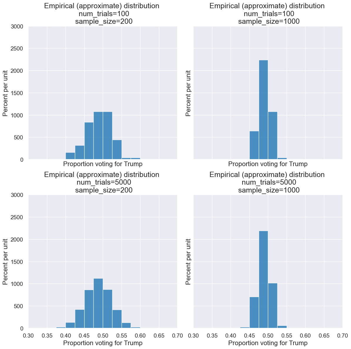
interact(simulate_and_plot_trump_pollster,
         num_trials = Choice(make_array(1,10,100,1000,5000)),
         sample_size = Choice(make_array(1,10,100,1000,5000)))
As another way to look at it, here’s an visualization showing the empirical distribution for a small sample size with varying numbers of trials.
And here’s one show showing the empirical distribution for varying sample sizes.
And here’s an animation showing the empirical distribution for varying sample sizes.
Big picture questions sampling:
Why wouldn’t we always just take really big of samples since they converge to the true distribution?
Big picture questions simulations:
What are we abstracting away when we’re writing code? What are we re-using over and over?