Table Examples
Contents
Table Examples#
Note: This notebook is set up to give you practice with the material we’ve covered so far this semester. The solutions to the questions posed on this page are visible if you show the hidden cells, but we encourage you to try to solve them on your own. You may do so on paper or by opening this notebook. It has blank cells for you to write the solutions to each question from scratch.
from datascience import *
from cs104 import *
import numpy as np
%matplotlib inline
1. Group and Pivot Practice#
Question. Write a function volume that takes the radii for some spheres as an array and returns the sum of the volumes of those spheres. Test your solution with several check operations.
Recall that the volume of a sphere with radius \(r\) is: \( \frac{4}{3} \pi r^3 \). Thus, the volume for a sphere with radius 1 is approximately 4.1888, and the volume when the radius is 2 is 33.5103.
def volume(radii):
    return sum(4/3 * np.pi * radii ** 3)

check(volume(make_array(1)) == approx(4.1888))
check(volume(make_array(1,2)) == approx(4.1888 + 33.5103))
Here is a small table with marble data.
marbles = Table().with_columns('Color', np.random.choice(['Red', 'Yellow', 'Blue'], 10),
                               'Transparency', np.random.choice(["Opaque", "Transparent"], 10),
                               'Radius', np.random.choice(np.arange(1,5), 10))
marbles.show(4)
| Color | Transparency | Radius |
|---|---|---|
| Yellow | Transparent | 3 |
| Yellow | Opaque | 4 |
| Red | Transparent | 2 |
| Yellow | Transparent | 1 |
... (6 rows omitted)
Question. Create a new table that shows the total volume of the marbles of each color. The columns of the new table should be ‘Color’ and ‘Volume’.
volumes = marbles.group('Color', volume)
volumes = volumes.relabeled('Radius volume', 'Volume')
volumes = volumes.select('Color', 'Volume')
volumes
| Color | Volume |
|---|---|
| Blue | 385.369 |
| Red | 335.103 |
| Yellow | 418.879 |
Question. Create a new table that shows the total volume of the marbles of each combination of color and transparency. Opaque or Transparent. The columns of the new table should be ‘Color’ and ‘Opaque’, ‘Transparent’, and there should be one row for each color.
marbles.pivot('Transparency', 'Color', 'Radius', volume)
| Color | Opaque | Transparent |
|---|---|---|
| Blue | 4.18879 | 381.18 |
| Red | 33.5103 | 301.593 |
| Yellow | 268.083 | 150.796 |
2. Hopkins Trees#
hopkins_trees = Table.read_table("data/hopkins-trees.csv")
hopkins_trees = hopkins_trees.drop("genus", "species")
hopkins_trees.sample(4)
| plot | common name | count |
|---|---|---|
| p0302 | Maple, sugar | 3 |
| p1032 | Maple, red | 72 |
| p0818 | Maple, red | 28 |
| p0016 | Maple, sugar | 30 |
Question. Create a table showing the number of trees of each species in whole forest, sorted from most to least.
tree_counts = hopkins_trees.drop("plot").group("common name", sum).sort("count sum", descending=True)
tree_counts = tree_counts.relabeled('count sum', 'count')
tree_counts.show(4)
| common name | count |
|---|---|
| Beech, American | 42922 |
| Maple, striped | 8939 |
| Maple, red | 5564 |
| Maple, sugar | 5193 |
... (73 rows omitted)
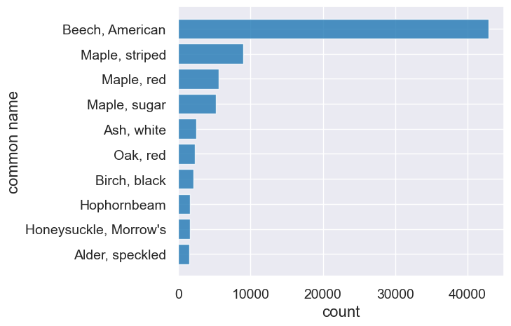
Question. Show the top ten tree species in a bar chart.
tree_counts.take(np.arange(0,10)).barh('common name', 'count')
Question. Create a table with counts for each type of maple for each plot. You should have a column for each species of Maple tree, and a row for each plot.
maples = hopkins_trees.where('common name', are.containing('Maple'))
maples.pivot('common name', 'plot', 'count', sum)
| plot | Maple, Norway | Maple, mountain | Maple, red | Maple, striped | Maple, sugar |
|---|---|---|---|---|---|
| p00-1 | 0 | 0 | 8 | 28 | 12 |
| p00-2 | 0 | 0 | 2 | 43 | 14 |
| p0000 | 0 | 0 | 13 | 0 | 4 |
| p0001 | 0 | 3 | 20 | 11 | 0 |
| p0002 | 0 | 0 | 12 | 1 | 0 |
| p0003 | 0 | 0 | 4 | 41 | 1 |
| p0004 | 0 | 0 | 2 | 9 | 3 |
| p0005 | 0 | 0 | 5 | 17 | 0 |
| p0006 | 0 | 0 | 3 | 26 | 14 |
| p0007 | 0 | 0 | 6 | 123 | 67 |
... (410 rows omitted)
Question. Make a histogram of the counts of red maples in each plot. Set bins to be np.arange(0,100,5) when creating the histogram.
red_maples = hopkins_trees.where("common name", are.equal_to("Maple, red"))
red_maples.show(3)
red_maples.hist('count', bins=np.arange(0,100,5))
| plot | common name | count |
|---|---|---|
| p00-1 | Maple, red | 8 |
| p00-2 | Maple, red | 2 |
| p0000 | Maple, red | 13 |
... (348 rows omitted)
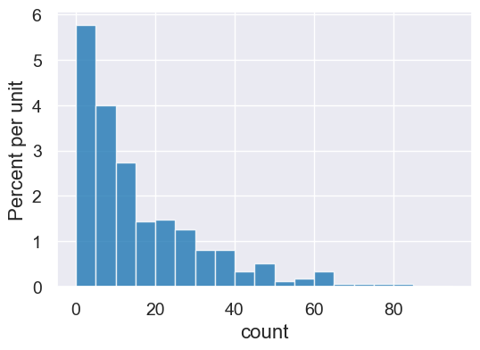
Questions about the plot you’ve created:
What are the units here?
How many plots have fewer than 10 red maples?
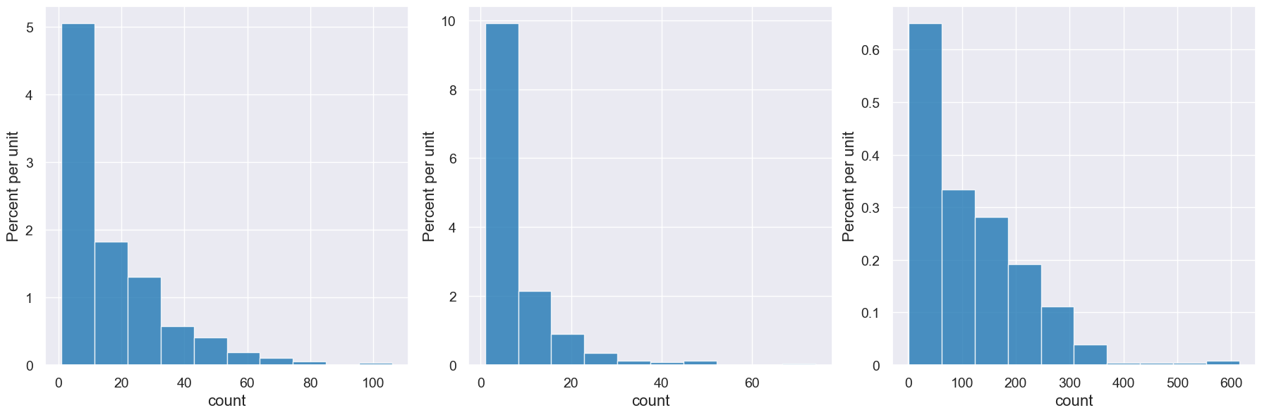
Question. Write a function that will produce a histogram of the counts of any given species in each plot.
def plot_counts(common_name):
    counts = hopkins_trees.where("common name", are.equal_to(common_name)).sort("count", descending=True)
    counts.hist('count')
with Figure(1,3):
    plot_counts('Maple, red')
    plot_counts('Oak, red')
    plot_counts('Beech, American')
Question. Write an interactive visualization that will show the histogram for the species selected from a popup menu.
all_names = hopkins_trees.sort('common name', distinct=True).column('common name')
interact(plot_counts, common_name=Choice(all_names))
3. Sky Scrapers#
Here’s a new dataset featuring skyscrapers in the US.
sky = Table.read_table('data/skyscrapers_v2.csv')
sky.show(5)
| name | material | city | height | completed |
|---|---|---|---|---|
| One World Trade Center | mixed/composite | New York City | 541.3 | 2014 |
| Willis Tower | steel | Chicago | 442.14 | 1974 |
| 432 Park Avenue | concrete | New York City | 425.5 | 2015 |
| Trump International Hotel & Tower | concrete | Chicago | 423.22 | 2009 |
| Empire State Building | steel | New York City | 381 | 1931 |
... (1776 rows omitted)
Question. Add an age column that indicates the age of each skyscraper in years.
sky = sky.with_column('age', 2025 - sky.column('completed'))
sky.show(3)
| name | material | city | height | completed | age |
|---|---|---|---|---|---|
| One World Trade Center | mixed/composite | New York City | 541.3 | 2014 | 11 |
| Willis Tower | steel | Chicago | 442.14 | 1974 | 51 |
| 432 Park Avenue | concrete | New York City | 425.5 | 2015 | 10 |
... (1778 rows omitted)
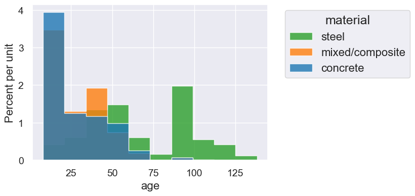
Question. Create an overlaid histogram of building age for the different materials. What does it tell you about skyscrapers?
sky.hist('age', group='material')
Question. For each city, what’s the tallest building for each material? Do it two ways: with group and with pivot.
tallest = sky.select('material', 'city', 'height').group(make_array('city', 'material'), max)
tallest.show(5)
| city | material | height max |
|---|---|---|
| Atlanta | concrete | 264.25 |
| Atlanta | mixed/composite | 311.8 |
| Atlanta | steel | 169.47 |
| Austin | concrete | 208.15 |
| Austin | steel | 93.6 |
... (86 rows omitted)
sky_pivot = sky.pivot('material', 'city', 'height', max)
sky_pivot.show(5)
| city | concrete | mixed/composite | steel |
|---|---|---|---|
| Atlanta | 264.25 | 311.8 | 169.47 |
| Austin | 208.15 | 0 | 93.6 |
| Baltimore | 161.24 | 0 | 155.15 |
| Boston | 121.92 | 139 | 240.79 |
| Charlotte | 265.48 | 239.7 | 179.23 |
... (30 rows omitted)
Question. For each city, what’s the height difference between the tallest steel building and the tallest concrete building?
sky_diff = sky_pivot.with_column(
    'difference',
    abs(sky_pivot.column('steel') - sky_pivot.column('concrete'))
)
sky_diff.show(5)
| city | concrete | mixed/composite | steel | difference |
|---|---|---|---|---|
| Atlanta | 264.25 | 311.8 | 169.47 | 94.78 |
| Austin | 208.15 | 0 | 93.6 | 114.55 |
| Baltimore | 161.24 | 0 | 155.15 | 6.09001 |
| Boston | 121.92 | 139 | 240.79 | 118.87 |
| Charlotte | 265.48 | 239.7 | 179.23 | 86.25 |
... (30 rows omitted)
Question. Show a map with heights of tallest in each city.
# Load in some useful geo information
cities = Table().read_table('data/uscities.csv').where('population', are.above(300000))
cities = cities.select('city', 'lat', 'lng')
cities.show(5)
| city | lat | lng |
|---|---|---|
| New York | 40.6943 | -73.9249 |
| Los Angeles | 34.1141 | -118.407 |
| Chicago | 41.8375 | -87.6866 |
| Miami | 25.784 | -80.2101 |
| Dallas | 32.7935 | -96.7667 |
... (141 rows omitted)
tallest = sky.select('material', 'city', 'height').group('city', max)
tallest = tallest.join('city', cities).select('lat', 'lng', 'city', 'height max')

points = tallest.with_columns('colors', 'blue',
                              'areas', tallest.column("height max"))
Circle.map_table(points).show()
(We haven’t done much with maps – you can use this as a reference for your own work, but we’d never ask you to create maps like this on, say, the midterm…)