Welcome

We type code in cells and then run them.

2 + 4

6

2 ** 4

16

days_in_week = 7
hours_in_week = days_in_week * 24
hours_in_week

168

We use libraries other people wrote

# Some code to set up our notebook for data science!

from datascience import *
from cs104 import *
import numpy as np
%matplotlib inline

We write code to manipulate and analyze data

Hopkins Forest tree survey

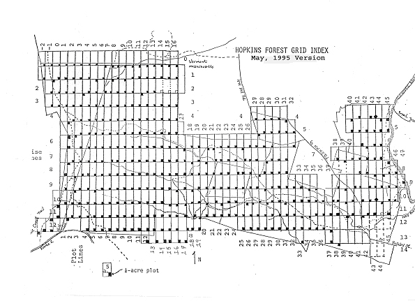
hopkins_trees = Table.read_table("data/hopkins-trees.csv")
hopkins_trees.show(10)

plot	genus	species	common name	count
p00-1	Acer	pensylvanicum	Maple, striped	28
p00-1	Acer	rubrum	Maple, red	8
p00-1	Acer	saccharum	Maple, sugar	12
p00-1	Amelanchier	canadensis	Shadbush	17
p00-1	Betula	alleghaniensis	Birch, yellow	7
p00-1	Betula	papyrifera	Birch, paper	5
p00-1	Fagus	grandifolia	Beech, American	142
p00-1	Ostrya	virginiana	Hophornbeam	7
p00-1	Prunus	serotina	Cherry, black	11
p00-1	Quercus	rubra	Oak, red	6

... (3783 rows omitted)

hopkins_trees = hopkins_trees.drop("genus", "species")
hopkins_trees  

plot	common name	count
p00-1	Maple, striped	28
p00-1	Maple, red	8
p00-1	Maple, sugar	12
p00-1	Shadbush	17
p00-1	Birch, yellow	7
p00-1	Birch, paper	5
p00-1	Beech, American	142
p00-1	Hophornbeam	7
p00-1	Cherry, black	11
p00-1	Oak, red	6

... (3783 rows omitted)

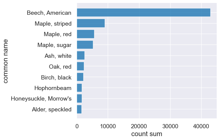
How many of each species?

hopkins_trees.drop("plot").group("common name", sum).sort("count sum", descending=True)

common name	count sum
Beech, American	42922
Maple, striped	8939
Maple, red	5564
Maple, sugar	5193
Ash, white	2523
Oak, red	2283
Birch, black	2144
Hophornbeam	1613
Honeysuckle, Morrow's	1608
Alder, speckled	1564

... (67 rows omitted)

tree_counts = hopkins_trees.drop("plot").group("common name", sum)
tree_counts = tree_counts.sort("count sum", descending=True)
tree_counts.take(np.arange(0,10)).barh("common name")

Where are all the red maples?

red_maples = hopkins_trees.where("common name", "Maple, red")
red_maples.sort("count", descending=True)

plot	common name	count
p0621	Maple, red	106
p1236	Maple, red	81
p0821	Maple, red	76
p1032	Maple, red	72
p0629	Maple, red	65
p1133	Maple, red	64
p1141	Maple, red	64
p0630	Maple, red	63
p0622	Maple, red	62
p0940	Maple, red	61

... (341 rows omitted)

But where are those plots?

plot_info = Table.read_table("data/hopkins-plots.csv").select("plot", "latitude", "longitude")
plot_info

plot	latitude	longitude
p00-1	42.7472	-73.2759
p00-2	42.7472	-73.2772
p0000	42.7472	-73.2747
p0001	42.7472	-73.2735
p0002	42.7472	-73.2723
p0003	42.7472	-73.271
p0004	42.7472	-73.2698
p0005	42.7472	-73.2686
p0006	42.7472	-73.2673
p0007	42.7472	-73.2661

... (413 rows omitted)

red_maples.join("plot", plot_info)

plot	common name	count	latitude	longitude
p00-1	Maple, red	8	42.7472	-73.2759
p00-2	Maple, red	2	42.7472	-73.2772
p0000	Maple, red	13	42.7472	-73.2747
p0001	Maple, red	20	42.7472	-73.2735
p0002	Maple, red	12	42.7472	-73.2723
p0003	Maple, red	4	42.7472	-73.271
p0004	Maple, red	2	42.7472	-73.2698
p0005	Maple, red	5	42.7472	-73.2686
p0006	Maple, red	3	42.7472	-73.2673
p0007	Maple, red	6	42.7472	-73.2661

... (341 rows omitted)

Visualization!

trees_with_lat_lon = hopkins_trees.join("plot", plot_info)

def population_map(tree_name):
    counts = trees_with_lat_lon.where("common name", tree_name)
    counts = counts.select("latitude", "longitude", "count")
    points = counts.with_columns("colors", "blue",
                                 "areas", 1.0 * counts.column("count")).drop("count")
    return Circle.map_table(points)

population_map("Maple, red")

Make this Notebook Trusted to load map: File -> Trust Notebook

Exploration, Hypotheses, and Drawing Conclusions

The following cell contains an interactive visualization. You won’t see the visualization on this web page, but you can view and interact with it if you run this notebook on our server here.

all_tree_names = np.unique(np.sort(trees_with_lat_lon.column("common name")))
interact(population_map, tree_name=Choice(all_tree_names))

Here are two examples of our iteractive map for different tree species

population_map("Birch, yellow")

Make this Notebook Trusted to load map: File -> Trust Notebook

population_map("Oak, red")

Make this Notebook Trusted to load map: File -> Trust Notebook

Even More Visualization

def population_choropleth(tree_name):
    counts = trees_with_lat_lon.where("common name", tree_name).select("plot", "count")
    return HopkinsForest.map_table(counts)

population_choropleth("Maple, red")

Make this Notebook Trusted to load map: File -> Trust Notebook