Hypothesis Testing

from datascience import *
from cs104 import *
import numpy as np
%matplotlib inline

1. Multiple Categories: Alameda Jury Panels

# data from ACLU study
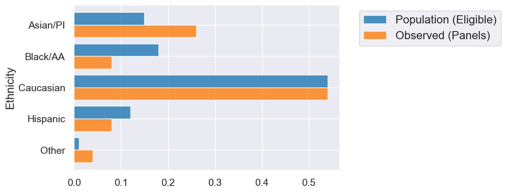
jury = Table().with_columns(
    'Ethnicity', make_array('Asian/PI', 'Black/AA', 'Caucasian', 'Hispanic', 'Other'),
    'Population (Eligible)', make_array(0.15, 0.18, 0.54, 0.12, 0.01),
    'Observed (Panels)', make_array(0.26, 0.08, 0.54, 0.08, 0.04)
)

jury

Ethnicity	Population (Eligible)	Observed (Panels)
Asian/PI	0.15	0.26
Black/AA	0.18	0.08
Caucasian	0.54	0.54
Hispanic	0.12	0.08
Other	0.01	0.04

jury.barh('Ethnicity')

eligible_population = jury.column('Population (Eligible)')

#What we see in the real-world data 
observed_sample_size = 1453

#Our simulation will use "sample proportions" function
sample_proportions(observed_sample_size, eligible_population)

array([0.1541638 , 0.18375774, 0.53475568, 0.11975224, 0.00757054])

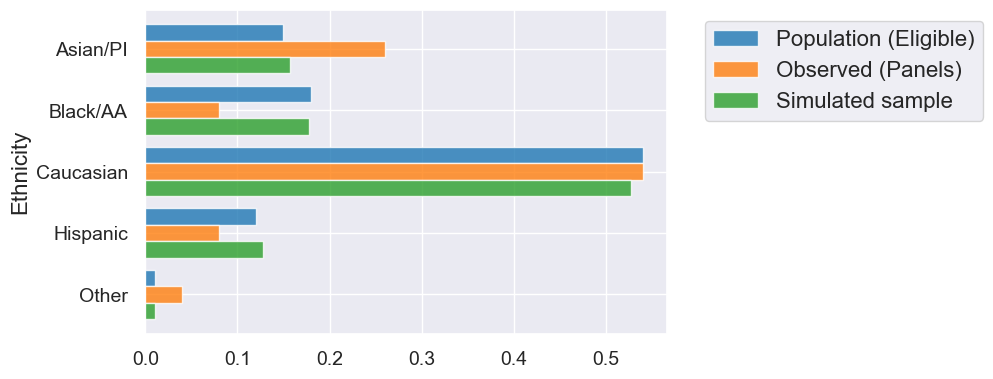
simulated_sample = sample_proportions(observed_sample_size, eligible_population)
simulated = jury.with_columns('Simulated sample', simulated_sample)
simulated

Ethnicity	Population (Eligible)	Observed (Panels)	Simulated sample
Asian/PI	0.15	0.26	0.153476
Black/AA	0.18	0.08	0.178252
Caucasian	0.54	0.54	0.538885
Hispanic	0.12	0.08	0.117688
Other	0.01	0.04	0.0116999

simulated.barh('Ethnicity')

TVD Statistic: Distance Between Two Distributions

jury.barh('Ethnicity')

jury_with_diffs = jury.with_columns(
    'Difference', jury.column('Observed (Panels)') - jury.column('Population (Eligible)')
)
jury_with_diffs

Ethnicity	Population (Eligible)	Observed (Panels)	Difference
Asian/PI	0.15	0.26	0.11
Black/AA	0.18	0.08	-0.1
Caucasian	0.54	0.54	0
Hispanic	0.12	0.08	-0.04
Other	0.01	0.04	0.03

jury_with_diffs = jury_with_diffs.with_columns(
    'Absolute Difference', np.abs(jury_with_diffs.column('Difference'))
)

jury_with_diffs

Ethnicity	Population (Eligible)	Observed (Panels)	Difference	Absolute Difference
Asian/PI	0.15	0.26	0.11	0.11
Black/AA	0.18	0.08	-0.1	0.1
Caucasian	0.54	0.54	0	0
Hispanic	0.12	0.08	-0.04	0.04
Other	0.01	0.04	0.03	0.03

sum(jury_with_diffs.column('Absolute Difference') / 2)

0.14

def total_variation_distance(distribution1, distribution2):
    return sum(np.abs(distribution1 - distribution2)) / 2

observed_panels = jury.column('Observed (Panels)')
total_variation_distance(observed_panels, eligible_population)

0.14

simulated_panel = sample_proportions(observed_sample_size, eligible_population)
total_variation_distance(simulated_panel, eligible_population)

0.023386097728836902

Simulating TVD Under the Model of Random Selection

def simulate_juries(observed_sample_size, num_trials):
    
    simulated_panel_tvds = make_array()
    
    for i in np.arange(0, num_trials):
        
        panel_sample = sample_proportions(observed_sample_size, 
                                          eligible_population)
        simulated_panel_tvd = total_variation_distance(panel_sample, 
                                                       eligible_population) #sample statistic is TVD 
        
        simulated_panel_tvds = np.append(simulated_panel_tvds, simulated_panel_tvd)
        
    return simulated_panel_tvds

num_trials = 3000
simulated_panel_tvds = simulate_juries(observed_sample_size, num_trials)
simulated_panel_tvds

array([0.00486579, 0.00883689, 0.01245699, ..., 0.01337233, 0.01227805,
       0.0223744 ])

Simulated versus observed

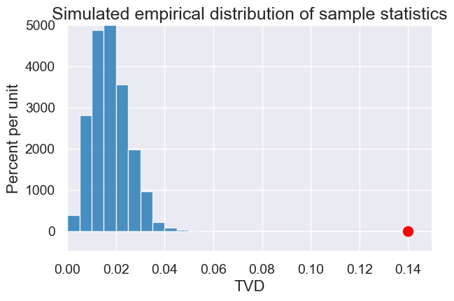
simulated_tvds = Table().with_column('TVD', simulated_panel_tvds)
plot = simulated_tvds.hist(bins=np.arange(0, 0.2, 0.005))

#Draw a red dot for the statistic on the observed (not simulated) data
observed_tvd = jury.column('Observed (Panels)')
observed_statistic = total_variation_distance(observed_tvd, eligible_population)
plot.dot(observed_statistic)

plot.set_title('Predicted TVD assuming random selection')
plot.set_xlim(0, 0.15)
plot.set_ylim(-5, 50)

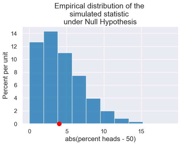
2. Is Coin Biased in Favor of Tails?

Recall, we create a simulation from our null hypothesis.

# Inputs to our hypothesis test simulation 
observed_num_flips = 100
null_hypothesis_proportions = make_array(0.5, 0.5)
observed_heads = 31

def plot_biased_coin_simulation(observed_num_flips, observed_heads, 
                           null_hypothesis_proportions, num_trials):
    
    #Null hypothesis model parameter which we will check against simulated
    null_hypothesis_percent_heads = 100 * null_hypothesis_proportions.item(0)
    
    #Simulate
    simulated_differences_from_null = make_array() 
    for i in np.arange(num_trials):
        coin_flips_sample = sample_proportions(observed_num_flips, 
                                               null_hypothesis_proportions)
        
        percent_heads = 100 * coin_flips_sample.item(0)
        abs_difference_from_null = abs(percent_heads - null_hypothesis_percent_heads)
        
        simulated_differences_from_null = np.append(simulated_differences_from_null, 
                                                    abs_difference_from_null)
    
    # Collect results 
    plot = Table().with_columns("abs(percent heads - 50)", 
                                simulated_differences_from_null).hist()
    
    # Draw a red dot for the statistic on the observed (not simulated) data
    observed_percent_heads = 100 * observed_heads / observed_num_flips
    observed_statistic = abs(observed_percent_heads - null_hypothesis_percent_heads)
    plot.dot(observed_statistic)
    
    plot.set_title("Empirical distribution of the \nsimulated statistic\n under the Null Hypothesis");

plot_biased_coin_simulation(100, 46, make_array(0.5, 0.5), 5000)

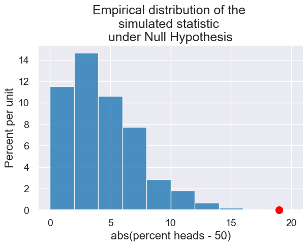
plot_biased_coin_simulation(100, 31, make_array(0.5, 0.5), 5000)

3. Midterm Scores

Was Lab Section 3 graded differently than that other lab sections, or could their low average score be attributed to the random chance of the students assigned to that section?

scores = Table().read_table("data/scores_by_section.csv")

scores.group("Section", np.mean)

Section	Midterm mean
1	15.5938
2	15.125
3	13.1852
4	14.7667

Lab section 3’s observed average score on the midterm

observed_average = np.mean(scores.where("Section", 3).column("Midterm"))
observed_average

13.185185185185185

Number of students in Lab Section 3

observed_sample_size = scores.group("Section").where("Section", 3).column('count').item(0)
observed_sample_size

27

Null hypothesis model: mean of the population

Null hypothesis restated: The mean in any sample should be close to the mean in the population

null_hypothesis_model_parameter = np.mean(scores.column("Midterm"))
null_hypothesis_model_parameter

14.727272727272727

Difference between Lab Section 3’s average midterm score and the average midterm score across all students

observed_statistic = abs(observed_average - null_hypothesis_model_parameter)
observed_statistic

1.5420875420875415

def sample_scores(sample_size):
    # Note: we're using with_replacement=False here because we don't 
    # want to sample the same student's score twice.
    return scores.sample(sample_size, with_replacement=False).column("Midterm")

def simulate_scores(observed_sample_size, num_trials):
    
    simulated_midterm_scores = make_array()
    
    for i in np.arange(0, num_trials): 
        
        one_sample = sample_scores(observed_sample_size)
        abs_difference_from_null = abs(np.mean(one_sample) - null_hypothesis_model_parameter)
        
        simulated_midterm_scores = np.append(simulated_midterm_scores, 
                                             abs_difference_from_null)

    return simulated_midterm_scores

simulated_midterm_scores = simulate_scores(observed_sample_size, 3000)

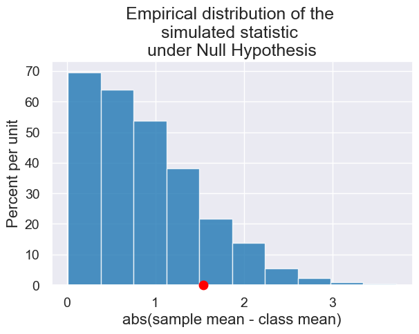
results = Table().with_columns("abs(sample mean - class mean)", simulated_midterm_scores)
plot = results.hist()    
plot.dot(abs(observed_average - null_hypothesis_model_parameter))
plot.set_title("Empirical distribution of the \nsimulated statistic \nunder Null Hypothesis");