Lab 6: Analyzing Precedent in the Supreme Court¶

Objectives

In this lab we will look at one of the most carefully curated social networks—the network of Supreme Court majority decisions. In doing so, you will gain experience with the following:

Using tuples and dictionaries
Sorting data
Plotting data using Python’s matplotlib library

Precedents in Supreme Court Decisions¶

In the US Supreme Court, the majority decision of a case is typically determined by citing past decisions. Past decisions establish precedent by being cited by later cases.

Citation network. Citing past work is also a common practice in academic publications. Publications establish legitimacy by citing related literature, and older publications become influential when they’re cited by future work. In academic circles, an author’s influence can be estimated by academic impact scores. In this lab we’ll attempt to apply a commonly-used academic impact score, called h-index, to dockets of Supreme Court decisions.

Getting Started¶

Before you begin, clone this week’s repository in the usual manner:

git clone https://evolene.cs.williams.edu/cs134-labs/22xyz3/lab06.git ~/cs134/lab06

where your CS username replaces 22xyz3.

You will find several CSV files in the data folder of your repository. The primary CSV file we will be using is data/judicial.csv. This file contains data that has been collected from Fowler and Jeon’s interesting analysis of the 30,288 majority US Supreme Court decisions on dockets (cases heard and decided by the Court in a session) through 2002.1

Each row in data/judicial.csv corresponds to a majority decision of the U.S. Supreme Court. There are many different columns, but we are primarily interested in the caseid (column 0), year (column 3), and indeg (column 8). The caseid column is a serial number the authors have given to each case in the order they were decided. The year column is the date of the decision. The indeg (or in degree) column is the number of later Supreme Court decisions that cite that particular case; we will refer to this statistic as the citation count for a decision. The data found in these three columns can be used to compute an impact score for each docket. In this context, you can think of a docket as a mapping from a year (int) to tuples of citation counts (ints) for each case heard that year.

For example, in the year 1783, there were three Supreme Court cases. You can verify this by searching for 1783 in the year column of data/judicial.csv. You will find 3 rows containing 1783 in the year column. Each row corresponds to a single case. Each of these cases had citation counts (indeg, column 8) of 0, 1, and 0 respectively. So the docket for 1783 is the tuple (0,1,0). For reference, these three rows are shown below.

41,1US72,,1783,0,0,0,0,0,0,0,20250,0,20945,0,0
42,1US73,,1783,0,0,0,0,1,0,0,20250,2.57E-05,15804,0,0.046963624
43,1US77,,1783,0,0,0,0,0,0,0,20250,0,20945,0,0

Part 0: Configuring your machine for matplotlib¶

IMPORTANT: Before starting this lab, you will need to have either installed matplotlib on your personal computer (as described in the setup guides of the course website), or you will need to setup and use a virtual environment. The lab machines are already configured for you.

Part 1: Analyzing Data¶

In this part, you will complete the functions in the file scotus.py to help interpret the data in judicial.csv.

Using CSV reader. In previous labs, we have directly read text files and processed the strings using standard string and list methods. In this lab, we will experiment with the csv module provided by Python to read more complicated CSV files. Start by reviewing the data/example.csv file. Notice that the name column includes first and last names separated by a ','. Thus simply splitting it across that character as we have done in previous labs will not work as intended. Instead, the csv module gives us a more robust way to interpret this kind of tabular data using a csv.reader() method. This method correctly splits the data by column into a list of strings even when commas are present in the data.

Experiment with the csv module in interactive Python as follows:
```
>>> import csv
>>> f = open("data/example.csv")
>>> data = csv.reader(f)
>>> type(data)
<class '_csv.reader'>
>>> for row in data:
...    print(row)
...
['id', 'name', 'office']
['rb17', 'Bhattacharya, Rohit', 'TBL-309B']
['jra1', 'Albrecht, Jeannie', 'TCL-305']
['sfreund', 'Steve Freund', 'TPL-302']
['lpd2', 'Doret, Lida', 'TCL-205']
```
Review scotus.py. Before writing any code, review the scotus.py module. Notice that we have given you the headers for each of the methods you must implement, as well as a few doctests associated with each method. We’ve marked places that require your attention with a pass statement; replace each pass with your own code. We have provided some initial doctests to help you debug, but you should also create your own additional tests as you evaluate your functions.

Reading the data of supreme-court decisions. We are ready to start coding! Start by implementing the function readDecisions(filename) in scotus.py. When given the filename data/judicial.csv, this method should read the contents of that CSV file using the csv.reader() method in the csv module as described above. It should create and return a new dictionary with integer years as keys and tuples of citation counts of cases heard that year (i.e., dockets) as values.

You may test the dictionary database returned by this function in the following ways:
```
>>> db = readDecisions('data/judicial.csv')
>>> db[1783]
(0, 1, 0)
>>> db[1784]
(1, 0, 1, 0, 0, 0, 0, 0, 1, 0)
>>> 1754 in db
True
>>> len(db[2002])
17
```
Computing the h-index. In academia, a commonly used metric for determining an author’s impact is the h-index. To compute an author’s h-index, we first count the number of times each of the author’s papers has been cited. An author’s h-index is defined as the maximum i where their top (most frequently cited) i papers have been cited at least i times.

For example, suppose Rita DeCoder has written ten papers. A tuple of her citation counts might look something like this:
```
(0, 2, 15, 9, 7, 48, 4, 82, 14, 6)
```
Rita’s first paper has been cited zero times, her second paper has been cited twice, her third has been cited 15 times, etc. Rita’s top 6 papers have each been cited at least 6 times, but the 7th is cited less than 7 times. Thus, Rita’s h-index is thus 6. This is more obvious when the tuple of citation counts is sorted in descending order:
```
(82, 48, 15, 14, 9, 7, 6, 3, 2, 0)
```
Authors with a high h-index have written many highly-cited papers and, over time, their impact score may improve as more and more people cite their works. For this lab, we will be computing the h-index of a specific Supreme Court docket, or more specifically, the h-index for a specific year as stored in your dictionary.

Implement the hIndex(citations) function in scotus.py. This function returns the h-index (int) of the tuple of citation counts provided. You probably will want to start by sorting your tuple of citation counts in some way, and using this is a basis for computing the h-index. The doctests provide some helpful examples. Make sure your code works correctly for these cases.
```
>>> hIndex( (1,3,4) )
2
>>> db = readDecisions('data/judicial.csv')
>>> db[1784]
(1, 0, 1, 0, 0, 0, 0, 0, 1, 0)
>>> hIndex(db[1784])
1
>>> db[1794]
(0, 3, 6, 5, 0, 0, 0, 0)
>>> hIndex(db[1794])
3
```
To demonstrate that your implementation of hIndex() is functional, please add two new doctests of your own design to the function.

Part 2: Plotting Data¶

Implement the function plotImpacts(dockets, plotFilename) in scotus.py. This method takes a docket database (a dict) and the name of the outputted plot file (a str). The function should plot impact (h-index) vs. docket year using line-style plotting to suggest trends. Be careful to correctly order your data points: construct a list of the years for which there are dockets, in ascending order. Then, use this list to generate a corresponding list of impact values.

You will want to use code similar to the following to actually generate the plot:
```
plt.title('The Title of Your Plot')
plt.xlabel('Independent variable description')
plt.ylabel('Dependent variable description')
plt.plot(years, impacts, 'b-')
plt.savefig(plotFilename)
```
When plotted correctly, the early years of data will have the following form:

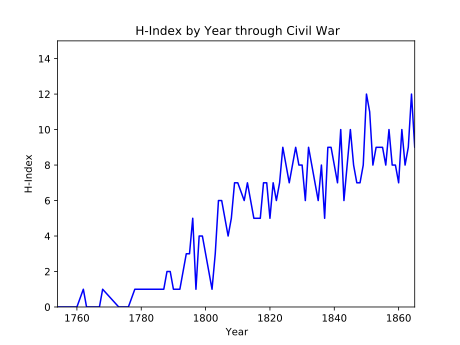
Your plot, of course, will be much more extensive, with more than 200 data points.

Part 3: Ranking Chief Justices¶

Now consider the file data/chiefJustices.csv. This file lists all the US Chief Justices along with the start and end year of their term. We can use this to rank the various courts (that is, the dockets of cases encountered while each Chief Justice was presiding) by their impact. Courts with high h-index values lead by setting precedent.

Implementing readCourts. Implement the method readCourts(justiceFilename, dockets) in scotus.py. Given a CSV file describing the Chief Justices called chiefJustices.csv, construct a mapping from the name of a justice to a tuple of cases heard while they were presiding. Each line of the CSV file contains a justice’s name followed by the start and end year of their term:
```
John Jay,1789,1795    
```
We should treat those years inclusively; it is fine if adjacent terms overlap.

Here’s how you might inspect this mapping in interactive Python:
```
>>> from scotus import *
>>> db = readDecisions('data/judicial.csv')
>>> courtDB = readCourts('data/chiefJustices.csv',db)
>>> jjCourt = courtDB['John Jay']
>>> len(jjCourt)
146
>>> max(jjCourt)
31
>>> jjCourt.index(31)
104
>>> hIndex(jjCourt)
5
```
Implement the rankJustices(courtDB) method. This method returns a list of (justice, impact) pairs (or tuples of two elements), sorted in decreasing order. This will require an understanding of the key option to the sorted() function. Recall that this optional parameter identifies a function that takes a tuple and returns the value used to rank that pair of values. In this case, we want to order these tuples by their second element, the court’s impact. We’ve provided a simple function, byImpact(), which you may find useful.

Here’s some code the demonstrates the use of rankJustices:
```
>>> from scotus import *
>>> dockets = readDecisions('data/judicial.csv')
>>> courtDB = readCourts('data/chiefJustices.csv',dockets)
>>> justiceRankings = rankJustices(courtDB)
>>> justiceRankings[-2]
('John Jay', 5)
```
The Jay Court did not see many cases, so it ranks close to the bottom in terms of overall impact.
Test your code. When the module’s methods are complete, you can run it as a script. Make sure you uncomment the final step (#5) in the if __name__ == "main" block. This will test your code and then print the various courts by decreasing impact.
```
python3 scotus.py
```
As always, make sure you add, commit, and push your work—scotus.py—to the server.

Submitting your work¶

When you’re finished, commit and push your work (scotus.py and honorcode.txt) to the server as in previous labs. (We will check to see that your script generates the desired plot; you need not submit the pdf file.)

Functionality and programming style are important, just as both the content and the writing style are important when writing an essay. Make sure your variables are named well, and your use of comments, white space, and line breaks promote readability. We expect to see code that makes your logic as clear and easy to follow as possible. Python Style Guide is available on the course website to help you with stylistic decisions.

Do not forget to add, commit, and push your work as it progresses! Test your code often to simplify debugging.

1: J. H. Fowler, S. Jeon, “The authority of Supreme Court precedent”, Social Networks, 30(1), January 2008, pp. 16-30.

CSCI 134: Introduction to Computer Science