How To Use Jupyter Notebooks¶

Jupyter notebooks allow us to have a rich web-based interface to interactive python. Moreover, they allow for documenting and visualizing programming projects. They are widely used as a presentation tool in the data science community. The name “Jupyter” is a loose acronym for Julia, Python and R: the programming languages that the application originally targeted.

This document gives you a brief overview of how to read, interpret and use Jupyter notebooks. If you have any questions, please contact the CSCI 134 staff.

Getting Started¶

You can run notebooks on your own computer in your Terminal window. If you are on a lab computer or followed our set up instructions for Macs or Windows, you everything should already be installed. If not, or you are unsure if you have install the software properly, simply run the following installation command in your terminal:

sudo pip3 install jupyterlab

In, the Terminal run the following command to start Jupyter:

jupyter lab

When you first launch Jupyter, you will see a landing page that looks like the following:

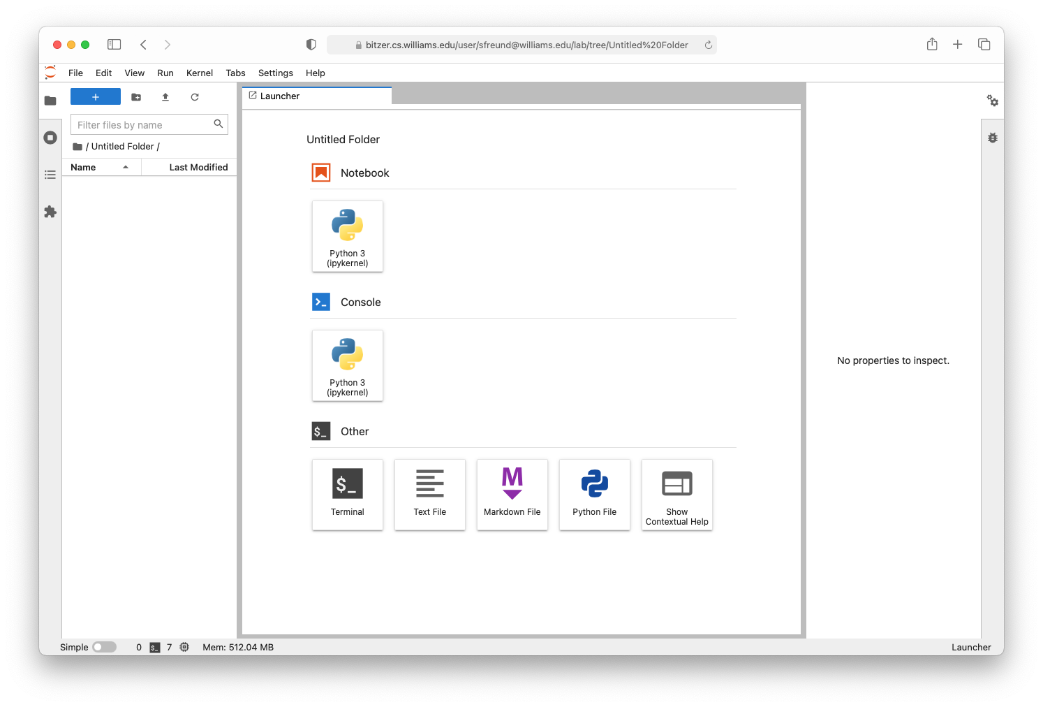
The window is divided into three panels:

The center panel enables you to create new notebooks for writing code interactively. Jupyter supports writing code in many different languages, but we’ll just stick to Python in 134.
The left panel shows the files in the directory where you ran jupyter lab, or the files on our server if you logged in there. You can navigate to and launch existing notebooks through this panel.
The right panel shows various properties of files you edit, but we won’t really do much with that. You can hide it by clicking the little gear icon in the top right corner of that panel.

The JupyterLab documentation covers the user interface in much more detail. The following tutorial should suffice for our needs.

Your First Notebook¶

Create a new notebook by clicking the “Python 3” button under Notebook in the Launcher window, or by selecting “File -> New -> Notebook” from the menubar. If Jupyter asks you to select the kernel, choose “Python 3 (ipykernel)”. A new tab should open up with a blank input cell:

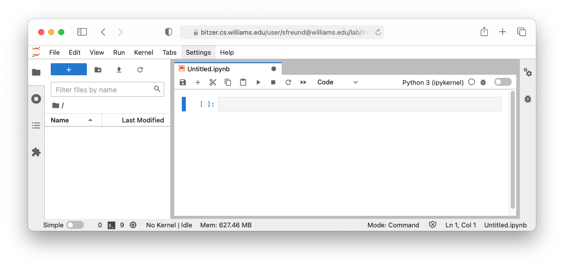
You can now type in snippets of Python code in the [ ] cell. For example, try typing 1+2:

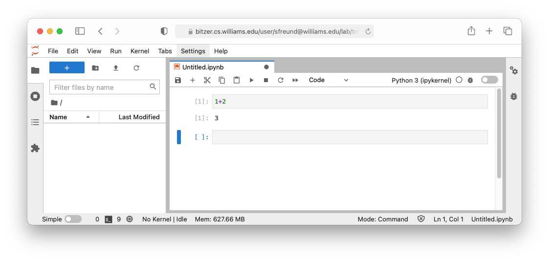
To run this code, select the cell (clicking on it will select it as seen by the blue highlight) and selected “Run -> Run Selected Cells” from the menubar. The keyboard shortcut to run cells is Shift+Enter (Mac) or Shift+Return (Windows). You should now see the output directly below with the label [1].

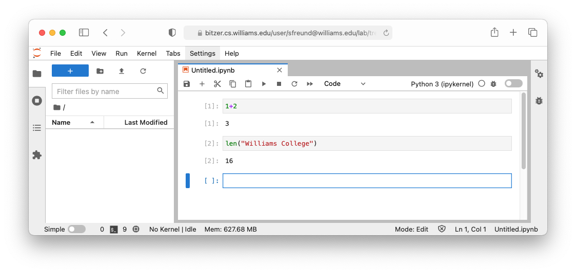
A new cell for more input should have appeard below the output line. You can always insert more cells by clicking the “+” in the toolbar at the top of the notebook tab. Type in some more python code and run it:

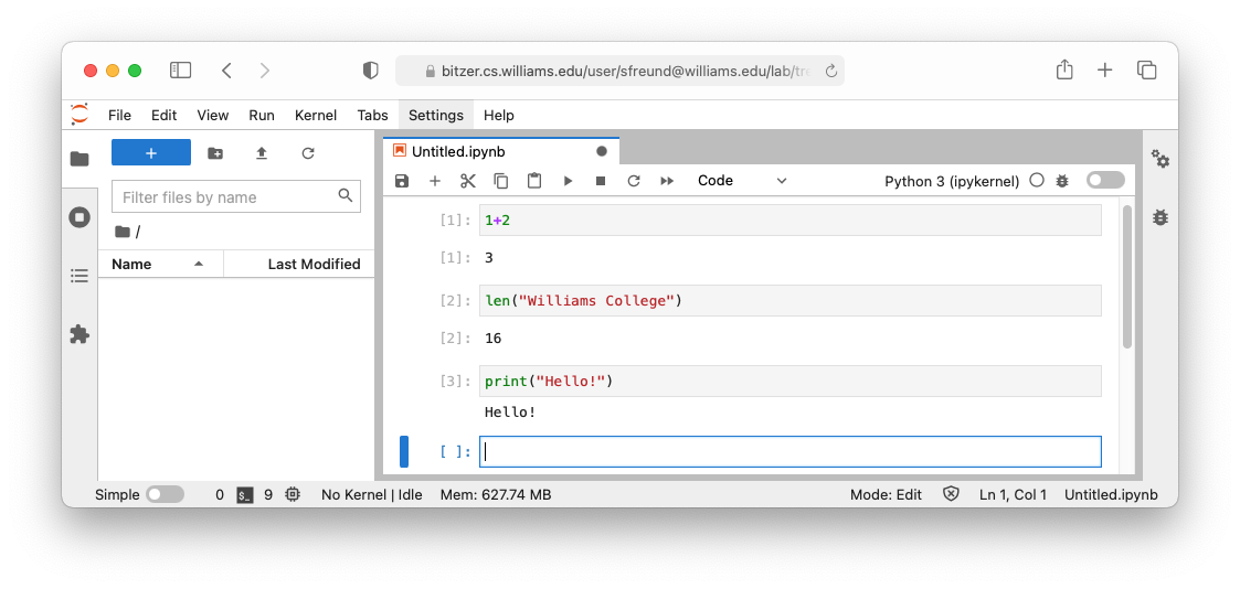
Note that typing a command in a cell in a Jupyter notebook is similar to typing it in an interactive Python session. When we “run the cell,” a number appears in the brackets to indicate that:
- the command has been executed, and
- the number n indicates that it is the nth command executed in the current session.
- In most cases, you can ignore this number. The output [n] cell of the notebook gives the resulting output.
Jupyter notebooks allow you to add rich notes along with examples. For example, you can change the “Cell Type” from Code to Markdown in the toolbar at the top of the tab to add Markdown-styled text.

Saving Your Notebook¶

When you are done, you can save the notebook by selecting “File -> Save Notebook” or “File -> Save Notebook As…” from the menubar. Note that if you are working on our sever, the notebook is stored there, not on your local computer. Selecting “File -> Download” from the menubar will let you download a copy of the file from our server to your own machine.

Quiting¶

To quit, select “File -> Logout” inside Jupyter, or simply close the browser tab running. If you launched Jupyter from a Terminal window, you’ll want to either close that window or press “Ctrl + C”.

Lecture Notebooks¶

We will be using Jupyter notebooks as a teaching aid in lectures. We’ll add links to those notebooks on the Calendar.

To view a notebook, simplly click on any Notebook link on the calendar, such as this one Notebook, which brings you to the notebook for Lecture 2. If all you wish to do is read the notes, you can simply browse through this page…

But you can also edit and run the notebook yourself:

First, be sure to have followed the setup instructions for Macs or Windows.
Then, click on the calendar for the day you are interested in. That will download a zip for with all of the materials for that lecture, including the notebook file. Save that file to an easily found location on your harddrive and unzip the contents.
Navigate to the directory containing the contents in the Terminal, and open the notebook by typing the following, where you should replace name-of-notebook with the actual name of the notebook you downloaded:
```
jupyter lab name-of-notebook.ipynb
```
You can execute each cell in the notebook one-by-one by selecting the cell and running it (via “Run -> Run Selected Cells” or Shift+Enter/Return). If you would like to execute all of them at once, you can select “Run -> Run All Cells”.
Feel free to add notes or extra examples to this notebook (and to lecture notebooks in general).