Confidence Intervals

from datascience import *
from cs104 import *
import numpy as np
%matplotlib inline

1. Pea plants

Population: all 2nd generation plants

Sample: Mendel’s garden: 929 plants, 709 which had purple flowers

Statistic: Percent Purple

Load Data

mendel_garden = Table().read_table('data/mendel_garden_sample.csv')
mendel_garden.show(4)

Plant Number	Color
0	Purple
1	Purple
2	White
3	White

... (925 rows omitted)

mendel_garden.num_rows

929

color_array = mendel_garden.column("Color")

Our statistic is the percent purple.

def percent_purple(color): 
    proportion = sum(color == "Purple") / len(color)
    return proportion * 100 

observed_stat = percent_purple(color_array)
observed_stat

76.31862217438106

Bootstrapping

Now we’re ready for our bootstrap_statistic function from our inference library.

results = bootstrap_statistic(color_array, percent_purple, 1000)

table = Table().with_columns("Bootstrap Samples Percent Purple", results)
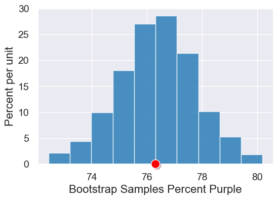
plot = table.hist("Bootstrap Samples Percent Purple")
plot.dot(observed_stat)

2. Confidence Intervals

Percentiles

tiny_purple_stat = make_array(78, 70, 88, 82)
tiny_purple_stat

array([78, 70, 88, 82])

percentile(50, tiny_purple_stat)

78

percentile(75, tiny_purple_stat)

82

Confidence Intervals for Pea Plants

ci_percent = 95

percent_in_each_tail = (100 - ci_percent) / 2
percent_in_each_tail

2.5

left_end = percentile(percent_in_each_tail, results)
left_end

73.51991388589882

right_end = percentile(100 - percent_in_each_tail, results)
right_end

78.90204520990312

This function, which is also in our inference library, computes the desired confidence interval for an array of statistics.

def confidence_interval(ci_percent, statistics):
    """
    Return an array with the lower and upper bound of the ci_percent confidence interval.
    """
    # percent in each of the the left/right tails
    percent_in_each_tail = (100 - ci_percent) / 2   
    left = percentile(percent_in_each_tail, statistics)
    right = percentile(100 - percent_in_each_tail, statistics)
    return make_array(left, right)

ci_95 = confidence_interval(95, results)
ci_95

array([73.51991389, 78.90204521])

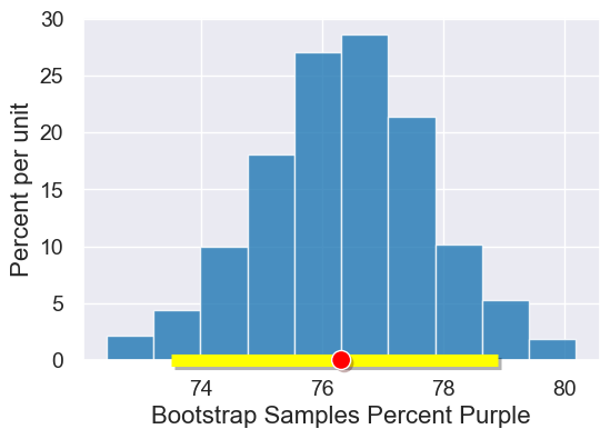
table = Table().with_columns("Bootstrap Samples Percent Purple", results)
plot = table.hist("Bootstrap Samples Percent Purple")
plot.interval(ci_95)
plot.dot(observed_stat)

Different Confidence Intervals

We can use confidence levels other than 95% too! Here is how the level impacts the size of the interval.

Our starting point:

confidence_interval(95, results)

array([73.51991389, 78.90204521])

If we’re okay with less confidence:

confidence_interval(90, results)

array([73.95048439, 78.68675996])

If we want more confidence:

confidence_interval(99, results)

array([72.7664155 , 79.97847147])

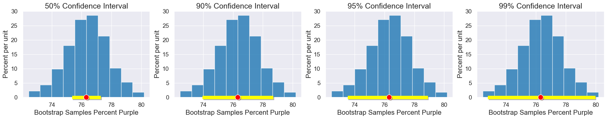
We can see the impact of confidence level on the width of the interval more easily in the plots below.

def visualize_ci(ci_percent):
    """
    Plot the desired confidence interval for our Mendel bootstrap run above.
    """
    table = Table().with_columns("Bootstrap Samples Percent Purple", results)
    plot = table.hist("Bootstrap Samples Percent Purple")
    plot.set_title(str(ci_percent) + "% Confidence Interval")
    plot.interval(confidence_interval(ci_percent, results))
    plot.dot(observed_stat)    

with Figure(1,4, figsize=(5,4)):
    visualize_ci(50)
    visualize_ci(90)
    visualize_ci(95)
    visualize_ci(99)    

The following cell contains an interactive visualization. You won’t see the visualization on this web page, but you can view and interact with it if you run this notebook on our server here.

interact(visualize_ci, ci_percent=Slider(0,100,1))

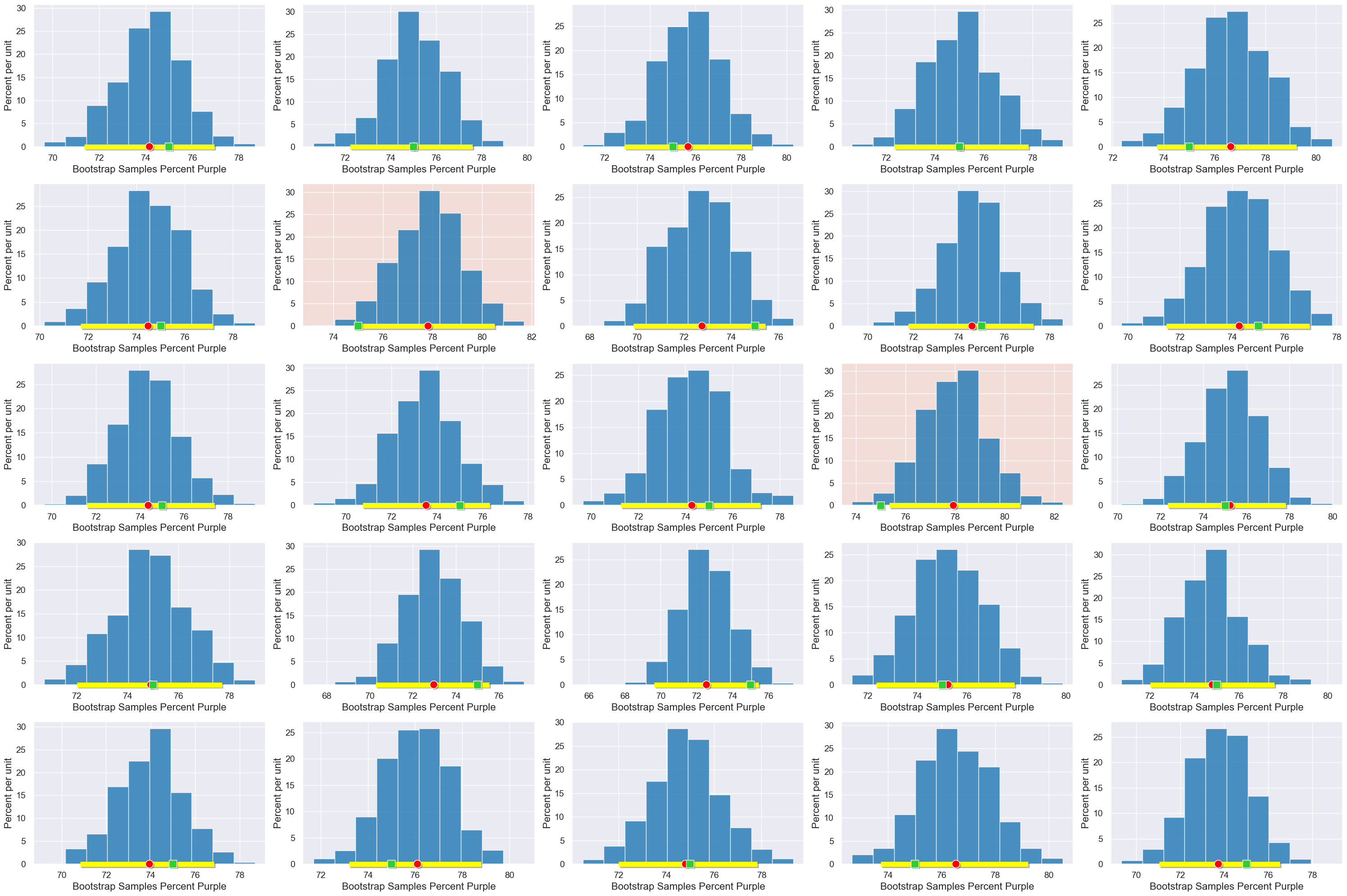
Interpreting Confidence

Here are 25 runs of our process on random samples. We expect 95% of our runs to produce confidence intervals containing the true parameter (75%).