Assessing Models
from datascience import *
import numpy as np
%matplotlib inline
import matplotlib.pyplot as plots
plots.style.use('fivethirtyeight')

import warnings
warnings.simplefilter(action="ignore", category=FutureWarning)
warnings.simplefilter(action="ignore", category=np.VisibleDeprecationWarning)

from ipywidgets import interact, interactive, fixed, interact_manual
import ipywidgets as widgets
1. Mendel and Pea Flowers
# Mendel owned 929 plants, of which 709 had purple flowers
observed_sample_size = 929
observed_purple_percent = 100 * (709 / observed_sample_size)
observed_purple_percent
76.31862217438106
# 3:1 ratio of purple:white, or 75% purple, 25% white
hypothesized_proportions = make_array(0.75, 0.25)
In the Python library reference, we see can use the function sample_proportions(sample_size, model_proportions).
peas_sample = sample_proportions(observed_sample_size, hypothesized_proportions)
peas_sample
array([0.75780409, 0.24219591])
Each item in the array corresponds to the proportion of times it was sampled out of sample_size times. So percent purple in sample:
simulated_purple_percent = 100 * peas_sample.item(0)
simulated_purple_percent
75.78040904198062
Let’s use our same simulation algorithm we return to over and over.
def simulate_purple_flowers(observed_sample_size, hypothesized_proportions, num_trials):

    simulated_purple_percents = make_array()

    for i in np.arange(0, num_trials):

        peas_sample = sample_proportions(observed_sample_size, hypothesized_proportions)
        # outcome: we only want the percent of the purple, we can drop the percent white
        simulated_purple_percent = 100 * peas_sample.item(0)

        simulated_purple_percents = np.append(simulated_purple_percents,
                                              simulated_purple_percent)

    return simulated_purple_percents
simulated_purple_percents = simulate_purple_flowers(observed_sample_size,
                                                    hypothesized_proportions,
                                                    1000)
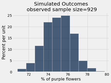
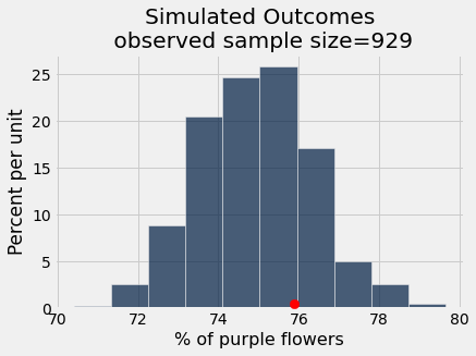
simulated_pea_results = Table().with_column('% of purple flowers', simulated_purple_percents)
simulated_pea_results.hist()
plots.title('Simulated Outcomes\n observed sample size=' + str(observed_sample_size));
Connecting these pieces together:
In Mendel’s model, he hypothesized getting purple flowers was like flipping a biased coin and getting heads 0.75 percent of the time.
We simulated outcomes under this hypothesis.
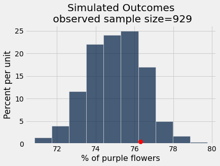
Now let’s check if the observed data (that there were 76.3% purple flowers in one sample, Mendel’s own garden) “fits” with the simulated outcomes under the model
simulated_pea_results.hist()
_ = plots.scatter(observed_purple_percent, 0.005, color='red', s=70, zorder=3)
plots.title('Simulated Outcomes\n observed sample size=' + str(observed_sample_size));
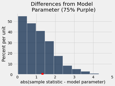
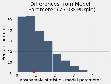
differences_from_model_parameter = Table().with_column('abs(sample statistic - model parameter)',
                                                       abs(simulated_purple_percents - 75))

differences_from_model_parameter.hist()
_ = plots.scatter(abs(observed_purple_percent - 75), 0.005, color='red', s=70, zorder=3);
plots.title('Differences from Model \n Parameter (75% Purple)');
Once again, let’s use computation to abstract away the variables that we have the power to change, and the parts of the code that never change.
def pea_plants_simulation(observed_sample_size, observed_purples_count,
hypothesized_purple_proportion, num_trials):
"""
Parameters:
- observed_sample_size: number of plants in our experiment
- observed_purples_count: count of plants in our experiment w/ purple flowers
- hypothesized_purple_proportion: our model parameter (hypothesis for
proportion of plants will w/ purple flowers).
- num_trials: number of simulation rounds to run
Outputs two plots:
- Empirical distribution of the percent of plants w/ purple flowers
from our simulation trials
- Empirical distribution of how far off each trial was from our hypothesized model
"""
# Make proportions for purple/white that match our hypothesized model.
observed_purple_percent = 100 * (observed_purples_count / observed_sample_size)
hypothesized_proportions = make_array(hypothesized_purple_proportion,
1 - hypothesized_purple_proportion)
# Simulate samples with same size as observed sample
simulated_purple_percents = make_array()
for i in np.arange(0, num_trials):
peas_sample = sample_proportions(observed_sample_size, hypothesized_proportions)
simulated_purple_percent = 100 * peas_sample.item(0)
simulated_purple_percents = np.append(simulated_purple_percents, simulated_purple_percent)
# Empirical distribution of sample statistics
simulated_pea_results = Table().with_column('% of purple flowers', simulated_purple_percents)
simulated_pea_results.hist()
_ = plots.scatter(observed_purple_percent, 0.005, color='red', s=70, zorder=10)
plots.title('Simulated Outcomes\n observed sample size=' + str(observed_sample_size));
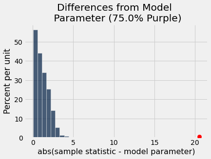
# Empirical distribution of differences between samples and observed
differences = abs(simulated_purple_percents - 100 * hypothesized_purple_proportion)
differences_from_model_parameter = Table().with_column('abs(sample statistic - model parameter)',
differences)
differences_from_model_parameter.hist()
_ = plots.scatter(abs(observed_purple_percent - 100 * hypothesized_purple_proportion),
0.005, color='red', s=70, zorder=10)
plots.title('Differences from Model \n Parameter (' + str(100 * hypothesized_purple_proportion) + '% Purple)');
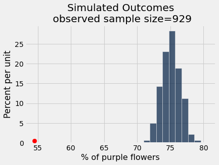
pea_plants_simulation(929, 705, 0.75, 1000)
pea_plants_simulation(929, 506, 0.75, 1000)
As an interactive visualization:
_ = widgets.interact(pea_plants_simulation,
                     observed_sample_size = fixed(929),
                     observed_purples_count = (0,929),
                     hypothesized_purple_proportion = (0,1,0.01),
                     num_trials=(10, 5000, 100))
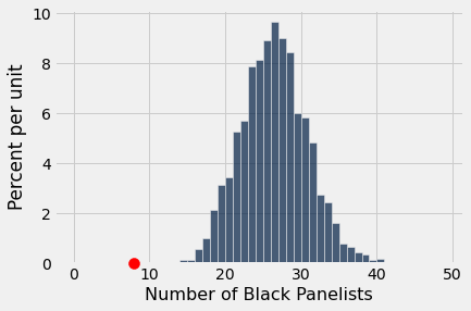
2. Single Category: Swain vs. Alabama
Eligible juror population at the time was men who were at 21 years old. In Talladega County, where the trial was held, 26% of the eligible jurors were Black. The 100-person panel of prospective jurors had 8 Black individuals. Should we expect this situation to happen frequently? Sometimes? Ever?
Need to sample from a categorical distribution (26% Black and 74% non-Black jurors) to create an emperical distribution of how many Black panelists to expect.
# define the population in terms of proportions
population_proportions = make_array(.26, .74)
population_proportions
array([0.26, 0.74])
# sample the population according to those proportions --> new library function!
sample_proportions(100, population_proportions)
array([0.25, 0.75])
def simulate_panel_selection(sample_size):
    """Return an array with the counts of [black, non-black] panelists in sample."""
    return np.round(sample_size * sample_proportions(sample_size, population_proportions))  # no fractional persons
simulate_panel_selection(100)
array([30., 70.])
def simulate_jury_panels(observed_sample_size, num_trials):

    simulated_black_panelists_counts = make_array()

    for i in np.arange(0, num_trials):

        panel_sample = simulate_panel_selection(observed_sample_size)
        simulated_black_panelists_count = panel_sample.item(0)   # count of panelists that are black

        simulated_black_panelists_counts = np.append(simulated_black_panelists_counts,
                                                     simulated_black_panelists_count)

    return simulated_black_panelists_counts
#Note: We want to create a simulation with the same conditions as the observed data
# So the samples in our simulation should be the same size as our observed sample size
simulated_black_panelists_counts = simulate_jury_panels(100, 3000)
simulated_black_panelists_results = Table().with_column('Number of Black Panelists',
                                                        simulated_black_panelists_counts)
simulated_black_panelists_results.hist(bins=np.arange(0,50))
#Draw a red dot for the statistic on the observed (not simulated) data
observed_black_panelists_counts = 8
plots.scatter(observed_black_panelists_counts, 0, color='red', s=100, zorder=10, clip_on=False);