JupyterHub

Contents

Inference with Statistics

# Some code to set up our notebook for data science!

from datascience import *
import numpy as np
%matplotlib inline
import matplotlib.pyplot as plots
plots.style.use('fivethirtyeight')

import warnings
warnings.simplefilter(action="ignore", category=FutureWarning)
warnings.simplefilter(action="ignore", category=np.VisibleDeprecationWarning)

from ipywidgets import interact, interactive, fixed, interact_manual
import ipywidgets as widgets

1. Snoopy’s Fleet

We will create a simulation for the empirical distribution of our chosen statistic.

At true inference time, we do not know N.

However, in our simulation we can make an assumption about what N might be so we can evaluate how “good” our chosen models and statistics could be.

# Our population.  Only Snoopy knows the population.  We don't.  All we can do
# is call `sample_plane_fleet` to observe planes flying overhead.

N = 300
population = np.arange(1, N+1)

def sample_plane_fleet(sample_size):
    """
    Return a random sample of planes from Snoopy's fleet.
    """
    return np.random.choice(population, sample_size)

sample = sample_plane_fleet(10)
sample

array([239,   3, 112, 181, 105, 165, 116, 271, 293,  15])

Option 1: Sample Statistic is the max plane number

# The outcome we care about is our chosen statistic evaluated on the sample 
# Chosen statistic option 1: max of sample 
outcome = max(sample)
outcome

293

Let’s put this all together using our simulation algorithm.

def simulate_plane_fleet(sample_size, num_trials): 
    all_outcomes = make_array()
    for i in np.arange(0, num_trials):
        sample = sample_plane_fleet(sample_size)
        outcome = max(sample)
        all_outcomes = np.append(all_outcomes, outcome)
    return all_outcomes

all_outcomes = simulate_plane_fleet(10, 1000)  # sample size is 10, num trials is 1000

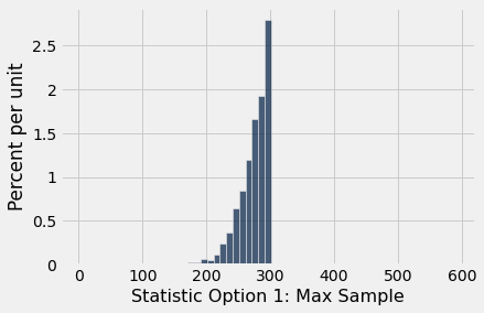
results = Table().with_columns("Statistic Option 1: Max Sample", all_outcomes)
results.hist(bins=np.arange(1, 2 * N, 10))

Let’s generalize a bit and create function that takes the statistic and runs the whole experiment

Option 2: Sample Statistic is Twice the Mean

Let’s generalize a bit and create function that takes the statistic and runs the whole experiment

def planes_empirical_statistic_distribution(sample_size, num_trials, statistic_function):
    """
    Simulates multiple trials of a statistic on our simulated fleet of N planes 
    
    Inputs 
        - sample_size: number of planes we see in our sample
        - num_trials: number of simulation trials 
        - statistic function: a function that takes an array 
            and returns a summary statistic (e.g. max)
        
    Output 
        Histogram of the results 
    """
    all_outcomes = make_array()
    for i in np.arange(0, num_trials):
        sample = sample_plane_fleet(sample_size)
        outcome = statistic_function(sample)
        all_outcomes = np.append(all_outcomes, outcome)
        
    results = Table().with_columns('Empirical Distribution, Statistic: ' + statistic_function.__name__, 
                                   all_outcomes)
    results.hist(bins=np.arange(1, 2 * N, 10))

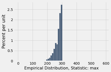
# sample size is 10, num trials is 1000, statistic is max
planes_empirical_statistic_distribution(10, 1000, max)

Our second option for the statistic:

def twice_mean(sample):
    """Twice the sample mean"""
    return 2 * np.mean(sample)

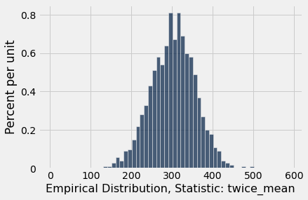
# sample size is 10, num trials is 1000, statistic is twice mean
planes_empirical_statistic_distribution(10, 1000, twice_mean)    

Effects of Sample Size and Simulation Rounds

def visualize_distributions(N, sample_size, num_trials):
    """A single function to run our simulation for a given N, sample_size, and num_trials."""
    population = np.arange(1, N+1)
    
    # Builds up our outcomes table one row at a time.  We do this to ensure
    # we can apply both statistics to the same samples.
    outcomes_table = Table(["Max", "2*Mean"])
    
    for i in np.arange(num_trials):
        sample = np.random.choice(population, sample_size)
        outcomes_table.append(make_array(max(sample), 2 * np.mean(sample)))
        
    outcomes_table.hist(bins=np.arange(1, 2 * N, 10))

_ = widgets.interact(visualize_distributions, N=(100, 500, 10), 
                     sample_size=(1, 100, 1), 
                     num_trials=(10, 5000, 100))

3. Mendel and Pea Flowers

# Mendel owned 929 plants, of which 709 had purple flowers
observed_sample_size = 929
observed_purples = 709 / observed_sample_size
observed_purples

0.7631862217438106

# 3:1 ratio of purple:white, or 75% purple, 25% white
hypothesized_proportions = make_array(0.75, 0.25)

In the Python library reference, we see can use the function sample_proportions(sample_size, model_proportions).

sample = sample_proportions(observed_sample_size, hypothesized_proportions)
sample

array([0.74058127, 0.25941873])

Each item in the array corresponds to the proportion of times it was sampled out of sample_size times. So percent purple in sample:

percent_purple = 100 * sample.item(0)
percent_purple

74.05812701829925

Let’s use our same simulation algorithm we return to over and over.

def simulate_purple_flowers(observed_sample_size, hypothesized_proportions, num_trials):
    
    all_outcomes = make_array()
    
    for i in np.arange(0, num_trials):
        
        simulated_sample = sample_proportions(observed_sample_size, hypothesized_proportions)
        # outcome: we only want the percent of the purple, we can drop the percent white
        outcome = 100 * simulated_sample.item(0)
        
        all_outcomes = np.append(all_outcomes, outcome)
        
    return all_outcomes

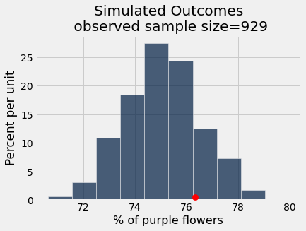
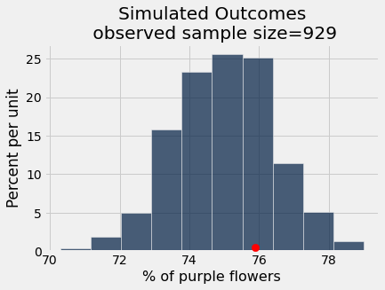
all_outcomes =  simulate_purple_flowers(observed_sample_size, hypothesized_proportions, 1000)

results = Table().with_column('% of purple flowers', all_outcomes)
results.hist()
plots.title('Simulated Outcomes\n observed sample size=' + str(observed_sample_size));

Connecting these pieces together:

• In Mendel’s model, he hypothesized getting purple flowers was like flipping a biased coin and getting heads 0.75 percent of the time.

• We simulated outcomes under this hypothesis.

• Now let’s check if the observed data (that there were 76.3% purple flowers in one sample, Mendel’s own garden) “fits” with the simulated outcomes under the model

results.hist()
_ = plots.scatter(100 * observed_purples, 0.005, color='red', s=70, zorder=3)
plots.title('Simulated Outcomes\n observed sample size=' + str(observed_sample_size));

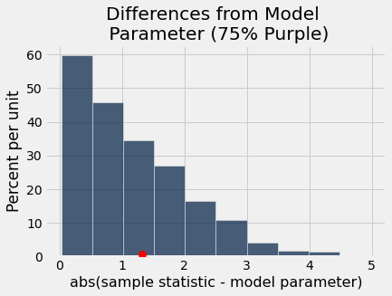
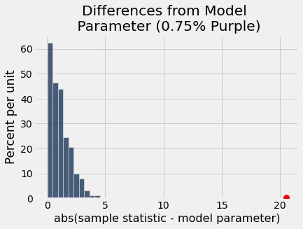
differences_from_model = Table().with_column('abs(sample statistic - model parameter)', 
                                             abs(all_outcomes - 75))

differences_from_model.hist()
_ = plots.scatter(abs(100 * observed_purples - 75), 0.005, color='red', s=70, zorder=3);
plots.title('Differences from Model \n Parameter (75% Purple)');

Once again, let’s use computation to abstract away the variables that we have the power to change, and the parts of the code that never change.

def pea_plants_simulation(observed_sample_size, observed_purples_count, 
                          hypothesized_purple_proportion, num_trials): 
    """
    Parameters:
        - observed_sample_size: number of plants in our experiment
        - observed_purples_count: count of plants in our experiment w/ purple flowers
        - hypothesized_purple_proportion: our model parameter (hypothesis for 
              proportion of plants will w/ purple flowers).
        - num_trials: number of simulation rounds to run
    Outputs two plots:
        - Empirical distribution of the percent of plants w/ purple flowers 
          from our simulation trials
        - Empirical distribution of how far off each trial was from our hypothesized model
    """
    
    observed_purples = observed_purples_count / observed_sample_size
    hypothesized_proportions = make_array(hypothesized_purple_proportion, 
                                         1 - hypothesized_purple_proportion)
    
    all_outcomes = make_array()
    for i in np.arange(0, num_trials):
        simulated_sample = sample_proportions(observed_sample_size, hypothesized_proportions)
        outcome = 100 * simulated_sample.item(0)
        all_outcomes = np.append(all_outcomes, outcome)
    
    #plots
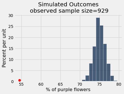
    percent_purple = Table().with_column('% of purple flowers', all_outcomes)
    percent_purple.hist()
    _ = plots.scatter(100 * observed_purples, 0.005, color='red', s=70, zorder=10)
    plots.title('Simulated Outcomes\n observed sample size=' + str(observed_sample_size));
    
    distance_from_model = Table().with_column('abs(sample statistic - model parameter)', 
                                              abs(all_outcomes - 100 * hypothesized_purple_proportion))
    distance_from_model.hist()
    _ = plots.scatter(100 * abs(observed_purples - hypothesized_purple_proportion), 
                      0.005, color='red', s=70, zorder=10)
    plots.title('Differences from Model \n Parameter (' + str(hypothesized_purple_proportion) + '% Purple)');

pea_plants_simulation(929, 705, 0.75, 1000)

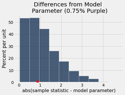
pea_plants_simulation(929, 506, 0.75, 1000)

As an interactive visualization:

_ = widgets.interact(pea_plants_simulation,  
                     observed_sample_size = fixed(929), 
                     observed_purples_count = (0,929), 
                     hypothesized_purple_proportion = (0,1,0.01),
                     num_trials=(10, 5000, 100))