Lab 5 : GraphViz [Optional]
Objective
- Utilize your ADT in a client app that lays out graphs visually.
Table Of Contents
Overview
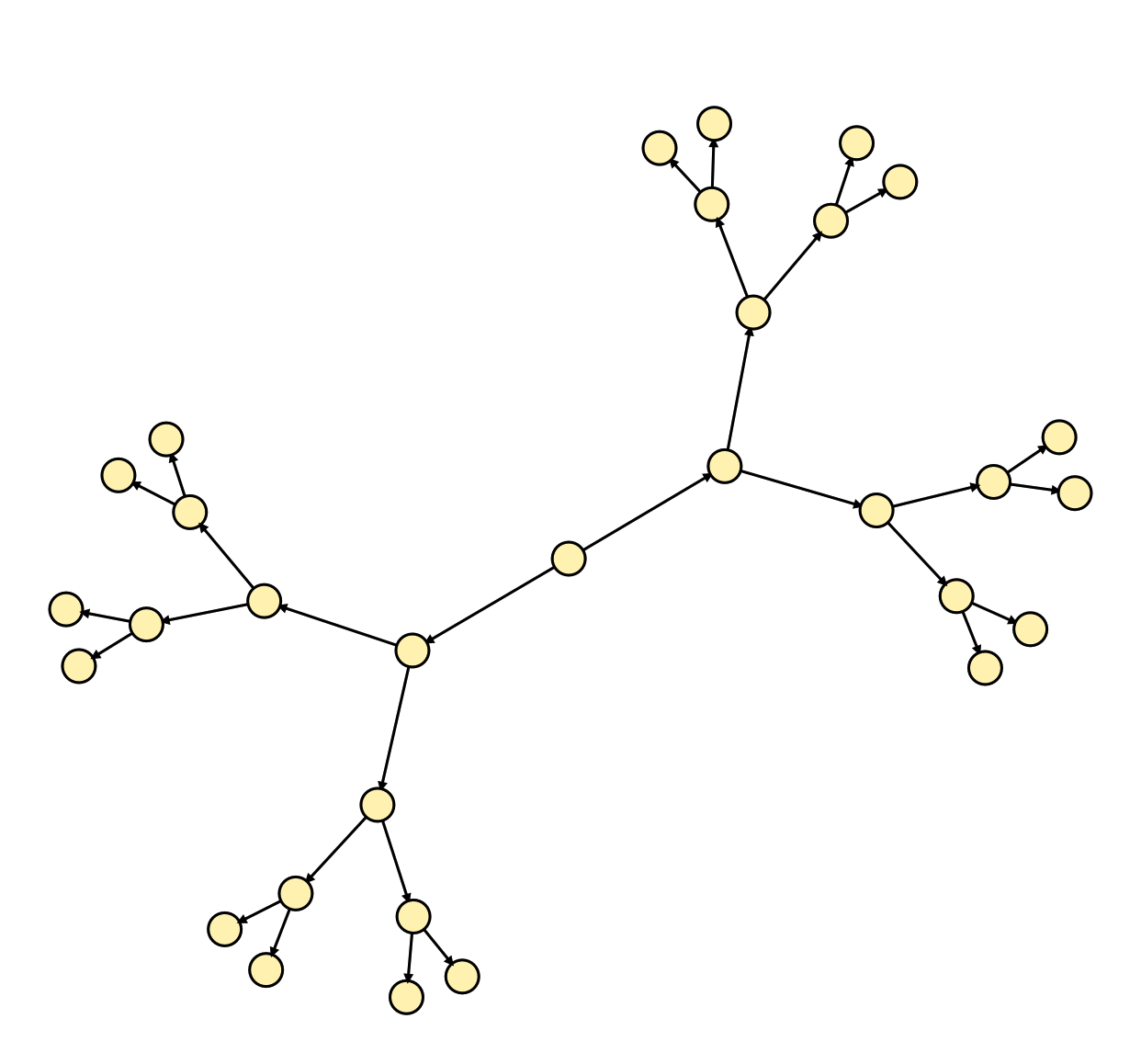
One nice property of graphs is that they have a natural geometric interpretation. For example, suppose that we want to represent friendships in a small group of people (A - E) using a graph. We could draw these relationships as edges between nodes (people) as follows:
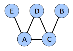
This is not the only possible way that we could have drawn this graph. Below are different renderings of the same graph:
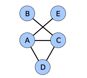
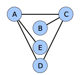
In all three of these cases, it is possible to discern the group’s friendships, but in the extreme, it is possible to lay out graphs in ways that entirely obscure the relationships between the graph’s nodes. For example, consider the following graph layouts:
The one on the right is for exactly the same graph as the left image, but the structure is much more visible. The drawing is symmetric, the nodes are spaced apart in an aesthetically pleasing manner, and the edges do not cross one another. This begs the question, “Given a graph, how can we produce an aesthetically good drawing for it?
GraphViz, the first client of your Graph, ADT will do just that using the force-directed layout algorithm described here.
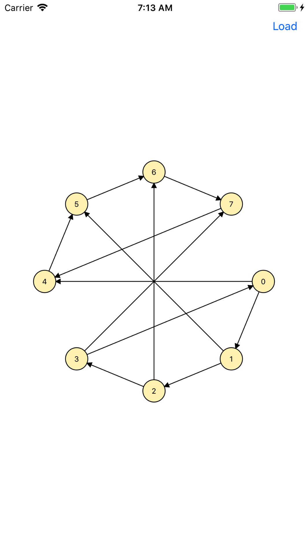
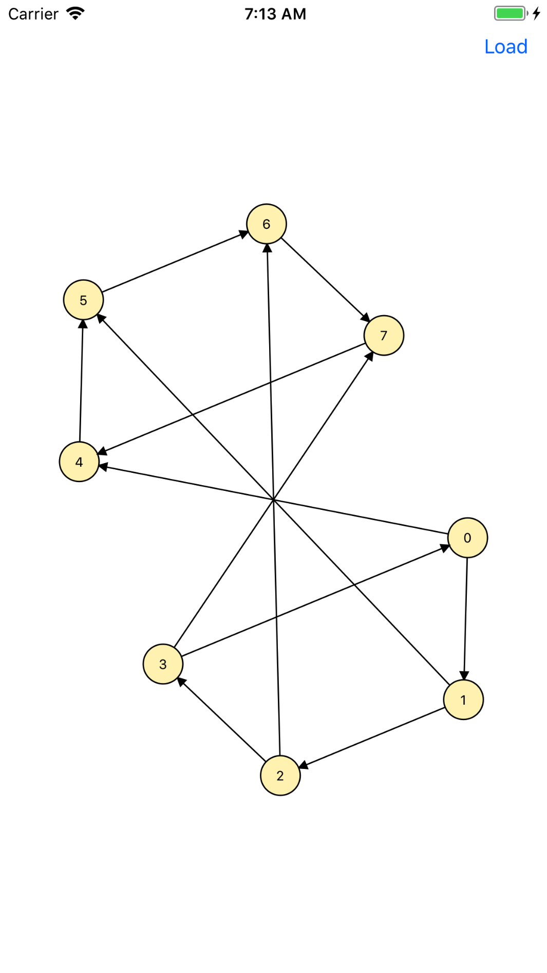
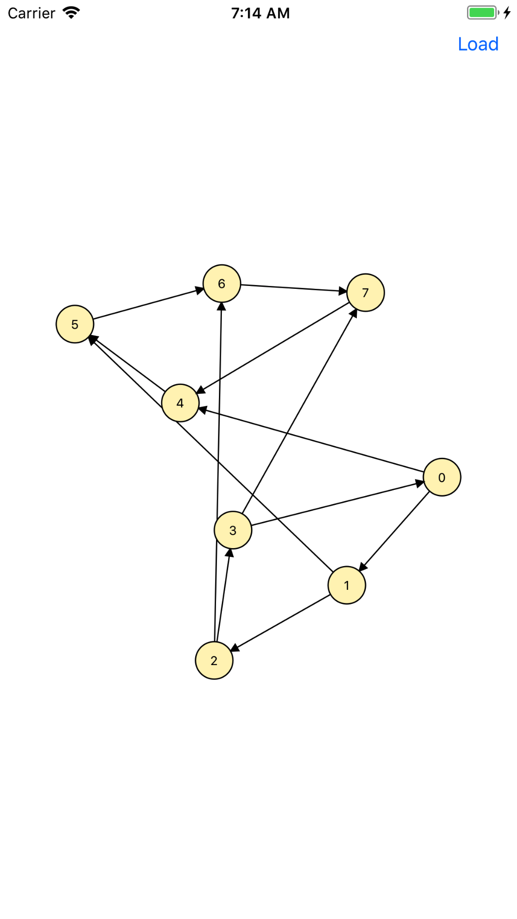
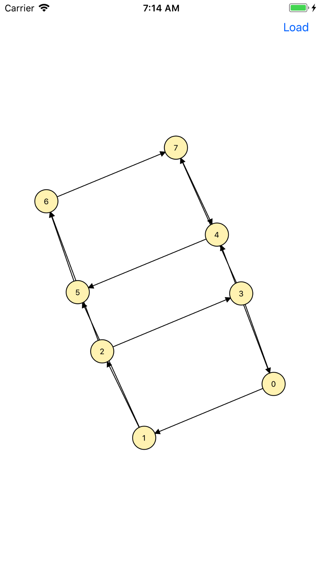
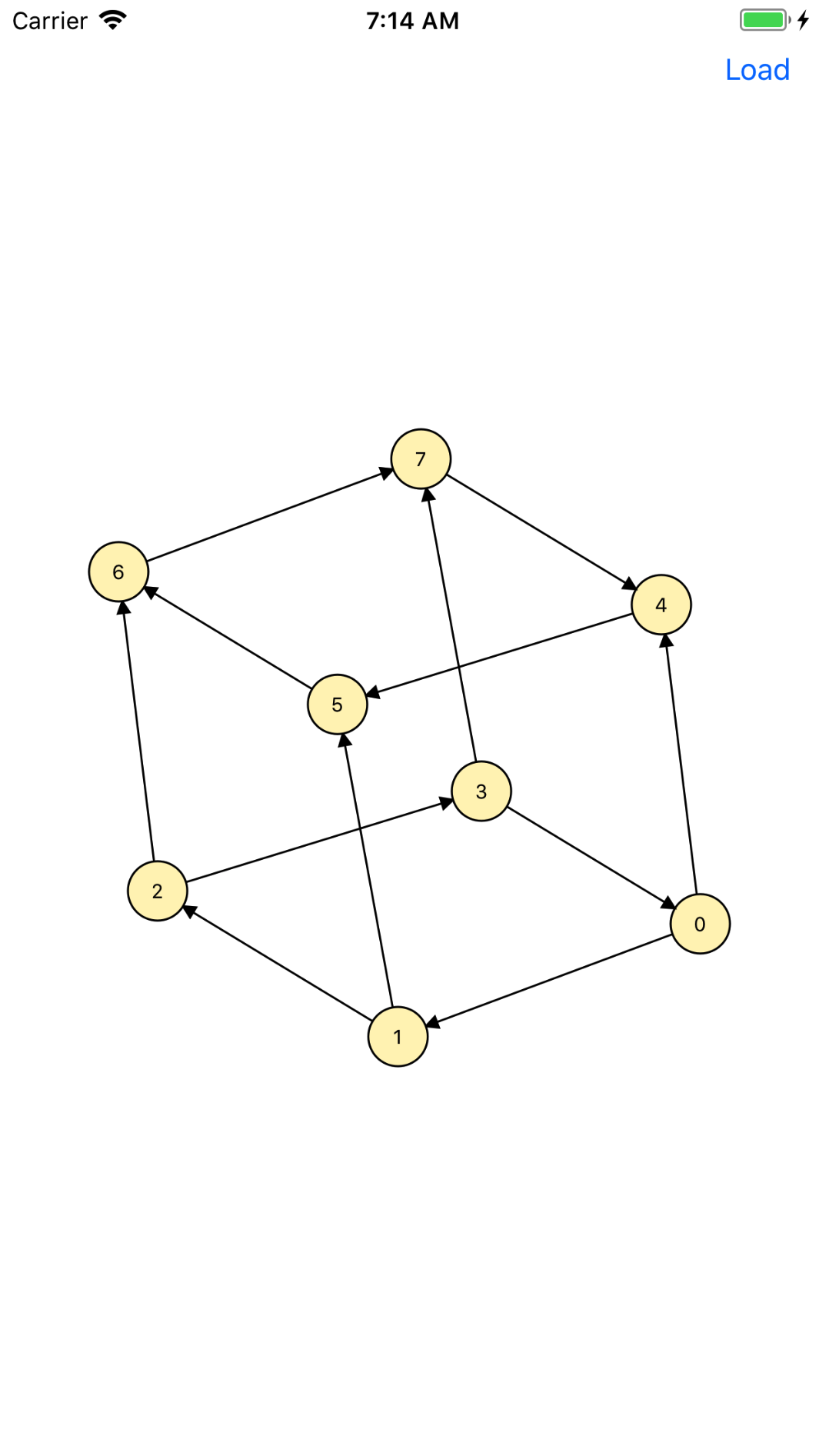
GraphViz loads graphs from JSON files and initially lays out the nodes in a circle. It then runs the force-directed algorithm, refreshing the view on each iteration, giving us an animation of how the notes are moved. Tapping the screen stops the animation until a new graph is loaded. Here are a series of screen shots taken as the app lays out a small graph:
Design and Implementation Plan
Problem 0: Understanding the Layout Algorithm
The graph drawing problem has been studied extensively. While there are many good algorithms for drawing graphs, no one algorithm shines as “the” graph drawing algorithm. Every algorithm has its strengths and weaknesses, and many algorithms that work well on certain graphs will produce poor layouts for other graphs. Before diving into the details of graph layout, we should decide what it means for a graph drawing to be “aesthetic pleasing”.
Layout Heuristics
We will use the following two common heuristics to guide how we will try to lay out graphs in an aesthetic pleasing way:
- Position connected nodes near one another. If connected nodes are near each other, a reader can focus on one part of the graph and see the local structure of the graph in that region. For example, below are two renditions of the same graph, where the graph on the left-hand side has connected nodes placed near each other and the right-hand side has connected nodes spaced far apart:
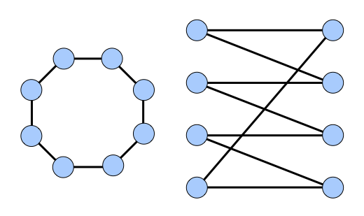
As you can see, the left-hand graph is much easier to interpret.
- Maximize the distance between unconnected nodes. If two unconnected nodes are placed near one another, the reader can be confused into thinking that they are somehow related when in fact there is no connection between them. For example, consider the two drawings below:
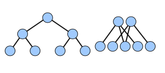
Again, the left-hand graph is much easier to interpret.
Algorithmically placing nodes according to these heuristics is difficult since the position of each node influences the position of each other node. Thus a direct approach requires solving a large, complex system of equations. However, there is an easier way for us…
Layout via Physics Simulation
Rather than solving for the answer directly, we’ll instead start with a random layout, then continuously refine the positions of the nodes to improve upon the heuristics. Over time, the nodes will reach a positions that balance the heuristics, and we’ll end up with an aesthetically pleasing graph drawing.
The key step in this algorithm is deciding how to update node positions, and to do this we’ll take a cue from physics. At each step of the graph layout, we’ll have the nodes exert forces on one another. These forces will push and pull nodes that are in sub-optimal positions until they eventually come to rest in a stable location. Because we want unconnected nodes to be far apart from one another, we’ll have each node repel each other node with some force. Similarly, because we want connected nodes to remain near one another, we’ll have each edge between nodes attract its endpoints. As these forces move the nodes around, the positions of the nodes will tend toward configurations where the net force on each node is minimized; that is, when there is a balance between the forces spacing out unconnected nodes and keeping together connected nodes.
- Assign each node in the graph an initial location.
- While the layout is not finished:
- Have each node exert a repulsive force on each other node.
- Have each edge exert an attractive force on its endpoints.
- Move the nodes according to the net force acting on them.
The details of each step is customizable: we can initialize the positions of the nodes however we choose, decide when the layout is good enough to stop, and use almost any function to determine the strengths of the attractive and repulsive forces. We’ll outline one set of design choices below, but we encourage you to try out your own variations; I’ve suggested several ideas at the end of this handout.
Assigning initial node positions. There is no one “correct way” to initially lay out the nodes in the graph. Because the algorithm takes an initial guess and improves over time, pretty much any initial layout will do, but some initial layouts will enable faster convergance. You’ll initially position the nodes so that they are evenly spaced apart on the unit circle. In particular, in a graph with \(n\) nodes, the \(k^{th}\) node should be placed at
\[ \left(\cos\frac{2 \pi k}{n},\sin\frac{2 \pi k}{n} \right)\]
Here, angles are represented in radians.
Determining when we’re finished. If the algorithm stops too early, then the nodes may not have moved into good positions; if it runs too long, the computer will waste time trying to improve upon an already perfect layout. There are ways to automatically detect whether to continue (or simply run for a fixed duration), but we’ll just let the user decide when to stop.
Computing forces. The particular approach we will use to compute forces is based on the Fruchterman-Reingold algorithm. In Fruchterman-Reingold, every node exerts a repulsive force on every other node that is inversely proportional to the distance between those nodes, and each edge exerts an attractive force on its endpoints proportional to the square of the distance between those nodes. This means that as connected nodes grow more distant to one another, the attractive force rises quickly and the repulsive force drops off, so connected nodes will have a tendency to “snap back” toward one another. Similarly, as the nodes draw increasingly close, the repulsive force grows rapidly while the attractive force diminishes, so the nodes will move away from each other. Only when the nodes are at a perfect distance from one another will the forces balance and the nodes cease to move.
To keep track of the net forces on each node \(a\), you’ll maintain \(\Delta x_a\) and \(\Delta y_a\) values storing the net forces on node \(a\) along the x and y axes. The net forces in each direction begin at zero, but will be adjusted by the interactions of each node with each other node:
Initial ForcesFor each node \(a\) at \((x_a, y_a)\):
- \(\Delta x_a = 0\)
- \(\Delta y_a = 0\)
The first source of force acting on each node is the repulsive force exerted by every node against every other node. For each pair of nodes \(a\) and \(b\) at positions \((x_a, y_a)\) and \((x_b, y_b)\), the magnitude of the repulsive force F_{repel} between these nodes is
\[ F_{repel} = \frac{k_{repel}}{\sqrt{ (x_b - x_a)^2 + (y_b - y_a)^2 }} \]
Where \(k_repel\) is a constant that controls the strength of the repulsive attraction. If the magnitude of this constant increases, then nodes repel each other more strongly; if it has a small magnitude, then nodes hardly repel each other at all. A value of \(0.005\) will work to get started, but you are free to experiment with this value if you wish.
Once you have computed the magnitude of the repulsive force, you will need to determine how much of that force is in the y-direction and how much of it is in the x-direction. To see how this force splits up, consider the following diagram:
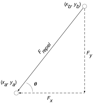
Here, \(F_x\) and \(F_y\) are the forces in the x and y directions exerted on the node at \((x_a, y_a)\). Using some simple trigonometry, we get that
\[ \begin{array}{rcl} F_{x_a} & = & −F_{repel} \cdot \cos \theta \\ F_{y_a} & = & −F_{repel} \cdot \sin \theta \end{array} \]
By Newton’s laws, the force exerted against the node \((x_b, y_b)\) are the opposite:
\[ \begin{array}{rcl} F_{x_b} & = & F_{repel} \cdot \cos \theta \\ F_{y_b} & = & F_{repel} \cdot \sin \theta \end{array} \]
Here, we’ve been using the angle \(\theta\) to represent the angle indicated in the above drawing. Again, simple trigonometry tells us that
\[ \theta = \tan^{-1} \frac{y_b - y_a}{x_b - x_a} \]
To summarize, the algorithm for computing repulsive forces is as follows:
Computing Repulsive ForcesFor each pair of nodes \(a\) and \(b\) at locations \((x_a, y_a)\) and \((x_b, y_b)\), respectively:
- Compute force and angle between nodes:
- \(F_{repel} = \frac{k_{repel}}{\sqrt{ (x_b - x_a)^2 + (y_b - y_a)^2 }}\)
- \(\theta = \tan^{-1} \frac{y_b - y_a}{x_b - x_a}\)
- Update forces on each node:
- \(\Delta x_a\)
-=\(F_{repel} \cdot \cos \theta\) - \(\Delta y_a\)
-=\(F_{repel} \cdot \sin \theta\) - \(\Delta x_b\)
+=\(F_{repel} \cdot \cos \theta\) - \(\Delta y_b\)
+=\(F_{repel} \cdot \sin \theta\)
- \(\Delta x_a\)
The second source of force acting on each node is the attractive forces between nodes joined together by edges. In this case, the attractive force \(F_{attract}\) is proportional to the square of the distance between the nodes:
\[ F_{attract} = {k_{attract}} \cdot ((x_b - x_a)^2 + (y_b - y_a)^2) \]
As above, \(k_{attract}\) is a constant controlling the strength of the attractive force and using the value \(0.005\) is a good starting point. Following similar reasoning as for repulsive forces, we can compute how this force divides over the x and y components as follows:Computing Attractive ForcesFor each edge from a node \(a\) at \((x_a, y_a)\) to a node \(b\) at \((x_b, y_b)\):
- Compute force and angle between nodes:
- \(F_{attract} = {k_{attract}} \cdot ((x_b - x_a)^2 + (y_b - y_a)^2))\)
- \(\theta = \tan^{-1} \frac{y_b - y_a}{x_b - x_a}\)
- Update forces on each node:
- \(\Delta x_a\)
+=\(F_{attract} \cdot \cos \theta\) // Note that this is+=, not-=! - \(\Delta y_a\)
+=\(F_{attract} \cdot \sin \theta\) - \(\Delta x_b\)
-=\(F_{attract} \cdot \cos \theta\) // Note that this is-=, not+=! - \(\Delta y_b\)
-=\(F_{attract} \cdot \sin \theta\)
- \(\Delta x_a\)
Moving Nodes According to the Forces. Once you’ve computed the net \(\Delta x_a\) and \(\Delta y_a\) forces for each node \(a\), moving the nodes is easy:
Moving NodesFor each node \(a\) at \((x_a, y_a)\):
- Move \(a\) to \((x_a + \Delta x_a, y_a + \Delta y_a)\)
(Note that in a true physical simulation the forces on each object would change the velocity of the object rather than directly modifying its position, but changing positions is sufficient. If you’d like to experiment with each node having a velocity and a position, feel free to do so.)
Problem 1: Project Setup
For this app, we will need to use your GraphADT Framework in another project. The easiest way to do this is to create an XCode “workspace” that includes both projects. A “product” from one (ie, your GraphADT.framework) can then be imported into the other. We have already set up the GraphProjects workspace for you in this way. Simply close the GraphADT project and instead open the GraphProjects.xcworkspace in your lab 5 directory. Once open, you should see both the GraphADT and GraphClients projects in the Project Navigator. The GraphClients project has a GraphViz target, which is what you will be working on. The Scheme options in the Tool bar should include targets from both projects, and you can build, test, and run either one from the workspace.
Even though the workspace is already set up, we’ll describe how to create it in case you ever need to something similar. Feel free to skip down to Problem 2: GraphViz Implementation.
Create a new workspace via “File -> New -> Workspace…”
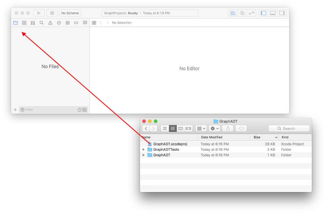
Then, find the XCode project you wish to include in Finder and drag the
.xcodeprojfile into the workspace’s Project Navigator, as illustrated below:
Repeat for each project you wish to include. Be sure they end up next to each other in the Project navigator, and not nested inside of each other. If that happens, simply drag the nested project to the top of the panel to reposition it.
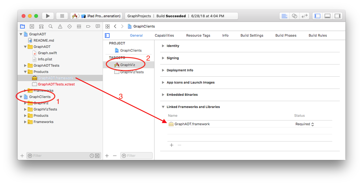
- To include a framework from one project in the target of another, select the General preferences for the target, and then drag the desired framework from the Project navigator into the list of “Linked Frameworks and Libraries”. For example, to add
GraphADT.frameworkto theGraphClients/GraphViztarget, follow the following steps:
Code from Connect The Dots
You will also need to add your GraphView.swift, GraphItem.swift (if a separate file), and ModelToViewCoordinates.swift files to the GraphViz target. I suggest doing this by first using the Finder to copy those source files from your ConnectTheDots project to the GraphProjects/GraphClients/GraphViz folder using the Finder. You can then add them to the GraphClients project selecting “Files -> Add Files to GraphClients…” from the menu bar inside XCode. (This avoids accidentally having your new project refer to the original versions of those files in the ConnectTheDots rather than new copies in GraphViz.) My solution to Connect The Dots is below – you may use these classes directly if you would like, or simply as guidance for design/style/documentation expectations.
- GraphView.swift
- GraphItem.swift
- ModelToViewCoordinates.swift
- DotPuzzle.swift
- ConnectTheDotsController.swift
And here is the jazzy-generated documentation.
Problem 2: GraphViz Implementation
You will need to implement GraphViz using the usual MVC design pattern. Plan your approach before you begin coding, and stage your development in small, manageable, and testable pieces. Be sure to look at the hints below as you begin working on this part.
Model
We have many choices for how to design the model for this program. In essence, we must keep a graph and the location where each node will be drawn. There are a number of design options here:
Change the graph ADT to keep a location for each node and have the graph manage layout; or
- Keep two variables in our controller:
var graph : Graphvar locations : [String:CGPoint]
and let the controller manage the layout.
Design a new class
DrawableGraphthat manages both the graph and the node locations inside of it, and that also provides methods for performing the layout steps. A minimal sketch of this class is as follows:public class DrawableGraph { private let graph : Graph = Graph() private var locations : [String:CGPoint] = [:] public init() { } public func add(_ node: String, at location: CGPoint) { ... add node to graph ... locations[node] = location } public func addEdge(from: String, to: String, label: String) { ... add edge to graph ... } public func location(of node: String) -> CGPoint { return locations[node]! } ... Any additional methods that are necessary to enable your ViewController to convert a DrawableGraph to an array of GraphItems and to run the layout algorithm... }This is the design I encourage you to follow.
Answer the following in the README.md for your GraphClients/GraphViz project.
Option 1 and 2 above both have shortcomings. Explain what they are in one or two sentences.
Explain how Option 3 avoids those shortcomings.
The JSON graph file format is different this week. Each file will have a nodes and edges section, with each edge having a source, destination, and label. Refer to the example files, such as small-cows.json, cows, and bull.json, for concrete examples. Most of the other data files just have empty edge labels since we are mostly interested in graph layout this week.
Layout Algorithm Code
I have also provided a skeleton of your Algorithm Steps 1, 3 and 4 so you don’t have to worry about implementing the mathematics. It’s not terribly difficult, but I’d like you to focus more on the other parts of the lab. My code uses a new Core Graphics struct, CGVector, to store \(\Delta\). Step 1 is implemented as a handy initializer that creates a DrawableGraph from a JSON file and evenly places the nodes around the unit circle, as described in Algorithm Step 1. Steps 3 and 4 are implemented as two distinct methods:
let forces = drawableGraph.computeForcesOnNodes()  // Algorithm Step 3
drawableGraph.moveNodes(by: forces)                // Algorithm Step 4
Note that you’ll need to fix up how my code accesses the DrawableGraph to match your own implementation.
As with all ADTs, include an abstraction function, representation invariant, and internal checkRep() method in your DrawableGraph class. To avoid repetition, you can simply refer to items from your Graph specification when appropriate. For example, the abstract state could simply be “same as the Graph’s abstract state, augmented with a location for each node”; the abstraction function can be “the graph described by the graph property, where the location of each node n is locations[n]”; and the rep invariant is that “locations has an entry for every node in graph”.
View
Your view will be a small extension over what you wrote for “Connect The Dots”. The new features you’ll support in your GraphView are the following:
Edges in our graphs are directed, and your
GraphViewshould indicate their direction by drawing edges as arrows. We have provided a method pathForArrow to create aUIBezierPathrepresenting an arrow. See the documentation for a description of the method parameters for customizing how the arrow path is created.Also, since edges are labeled in our graphs,
GraphItem.edgenow contains a label property.public enum GraphItem { case node(loc: CGPoint, name: String, highlighted: Bool) case edge(src: CGPoint, dst: CGPoint, label: String, highlighted: Bool) }Your
GraphViewclass should draw that label centered on theUIBezierPathcreated for the edge. (See the documentation for UIBezierPath.bounds to help with this. Once you get the path’s bounds, you can just get themidXandmidYof that CGRect to get the center of the path.)
Controller
The controller will have much of the same structure as in “Connect The Dots”, with a few notable exceptions:
The model will be a
DrawableGraph, and not aDotPuzzle, andupdateUI()will need to operate on thatDrawableGraph.When animating layout, remember that you should never block the main UI thread for long-running operations, such as adjusting node locations, and you must always perform any operation touching GUI components from the main UI thread. This requires special care. We’ll cover this in detail in class.
Also, you should stop the layout animation if the user loads a new file – otherwise you may end up trying to change the locations of nodes in the wrong graph.
Problem 3: Specification and Implementation Tests
Write any additional tests that would help you test your DrawableGraph model. Focus only on tests for new functionality in DrawableGraph. That is, don’t test everything you already tested for in your Graph tests, only in how your DrawableGraph uses the Graph. You may also assume the all of the code I give you is correct – there are some interesting ways to test implementations of this sort of algorithm, but we’re already doing more than enough for one week.
Overall, there may be little to do here. It may be as simple as writing a test or two to create small DrawableGraphs and ensuring that you can iterate over them and access node locations properly.
Your parts of the view and controller code should be a relatively small and self-contained part of your program that can be manually tested once you have tested your model.
Hints
Getting Started
You should be sure that graphs can be drawn correctly before working on the layout algorithm. That is, update your
GraphItemandGraphView, to display arrows and edge labels. You can test these changes with a View Controller that just generates creates a small array ofGraphItemsto give to the graph view inupdateUI().Once that works, you can extend the View Controller to load graph files, create
DrawableGraphs, and display the appropriate graph items in the view. This will look very much like your Connect The Dots controller.Two Interface Builder pitfalls to avoid while creating your UI:
When adding gesture recognizers, be sure to drag them from the object library onto the view that they should be enabled for.
To use a custom view, do not change the class of the root view for your UIViewController. Instead, draw a “View” object from the object library onto the view controller’s window, resize it to fit the whole window, and then change the class of that new view. If your gesture recognizer actions do not run, make sure this is set up properly.
Layout Algorithm
You may wish to initially have your controller perform one layout step on each tap, so you can debug your code and verify it works without animation. Adding animation should follow our example from class.
Since layout will change where nodes are positioned, after each layout step, you should perform the “Zoom To Max” operation to keep the entire graph visible.
Try out different input graphs – there are a lot, so you may need to scroll up and down in the pop-up action sheet to see them all when loading. If performance is slow on the larger ones, you can turn off your
checkRep()checks, as I showed in the slides for the testing/debugging lectures. We can help diagnose performance bottlenecks if you encounter any hitches along the way. Some of the extensions will also dramatically speed things up.
viewDidLoad() and viewDidLayoutSubviews()
- Your controller’s
viewDidLoad()method is a good place to load a file to start with. If you do this and find that the graph does not fill the screen even after “Zooming To Max”, it is likely that yourviewDidLoad()code runs before your views are fully layed out. You can fix this by including the following method, which runs after the controller lays out its views:
override func viewDidLayoutSubviews() {
    super.viewDidLayoutSubviews()
    self.graphView.zoomToMax() // or your equivalent method.
}
Extras
Our basic layout algorithm is one of many algorithms that can be used to draw graphs. Here are a few possible extensions to our basic technique you can to experiment with. I hope that you try at least one of these changes out, since most of them require only a few lines of code and can yield noticeable changes in the resulting graphs:
Change the relative strength of the attractive and repulsive forces. The algorithm uses two constants, \(k_{attract}\) and \(k_{repel}\), which control how strong the attractive and repulsive forces are. My suggestion is to set both of these values to \(0.005\) initially, but there’s no reason that they stay at this value, or that they even stay in a 1:1 ratio. Try changing these values independently of one another. What do you notice happening to the graph layouts? Do any values cause the algorithm to completely fail to work?
Add random perturbations. One potential problem with this force-directed algorithm is that the graph can get stuck in a local minimum, a configuration in which all of the forces are balanced but which is not the optimal configuration. Often, this manifests itself in a situation in which if any of the nodes were to move even a slight amount, the graph would collapse into a much better configuration. For example, consider a graph in which three nodes are each connected to one another in a triangle. One possible layout for the graph would be to put them all in a straight line. If this happens, then the repulsive and attractive forces on the nodes would always push and pull along that line, and so the nodes would always be collinear. However, if one of the nodes were to get bumped slightly out of place, then the forces between the nodes would no longer be along a line and the nodes will quickly arrange themselves in a triangle. Try modifying the current algorithm by giving each node a slight “push” in a random direction at each step of the process. Does this result in better layouts in any cases?
Add node velocities. In our force-directed algorithm, the amount each node moves on each iteration is completely independent of the amount that the node moved on the previous steps. That is, if a node moves a great distance on one step, it has no “memory” of this and on the next step it will move based solely on the current configuration. In an actual physical system, each node would have an associated velocity which would keep it moving in a particular direction until the net forces slowed it down. Consider modifying the algorithm to incorporate information about the previous iteration’s velocities into the current step. One way to do this would be to track the \(\Delta x\) and \(\Delta y\) of each object from one iteration to the next, rather than resetting it to zero each time. What do you notice about the graph layouts?
Add penalties for crossing edges. One aspect of graph drawings we did not take into account when computing forces is the number of edges that are crossing in a particular drawing. A graph drawing without crossings is more likely to be aesthetically pleasing than a graph drawing with crossings. Modify the algorithm to detect these crossings and adjust the layout accordingly. One common approach for doing this is to pretend that there is an invisible node at the center of each edge that exerts a repulsive force against the center of each other edge, thus pushing edges apart from one another.
Add penalties for low resolution. The resolution of a graph drawing is the smallest angle between any two edges incident to a single node. Graphs that have low resolution can be hard to understand, since the edges emanating from a source node will all be bunched together. Modify the algorithm to try to avoid low resolution. One way to do this might be to add a repulsive force between the endpoints of arcs that have a small angle between them.
Generalize the definition of an attractive force. In our current algorithm, only nodes directly connected by edges have an attractive force between them. The rationale behind this was that nodes that are connected to one another ought to be close to each other. However, given this same reasoning, it also makes sense to have nodes that are almost connected to one another exert a force on each other. For example, if node A is connected to node B and node B is connected to node C, then A and C are likely to be near each other in the nal graph layout. Similarly, if C is then connected to D, perhaps A and D should be near each other as well. Update the algorithm so that nodes that are more than one hop away from each other still exert an attractive force. One option might be to have each node exert an attractive force on each other node proportional to how “close” they are to one another in the initial graph.
There are a whole host of extensions you could try out, so don’t be limited just by these.
Add a small section describing any extras to your GraphClients/GraphViz/README.md file so we know what to look for.
Acknowledgement: Part this assignment utilizes material originally developed by Keith Schwartz.