Lab 5 Graph Layout Algorithms

• Layout Heuristics
• Layout via Physics Simulation

The graph drawing problem has been studied extensively. While there are many good algorithms for drawing graphs, no one algorithm shines as “the” graph drawing algorithm. Every algorithm has its strengths and weaknesses, and many algorithms that work well on certain graphs will produce poor layouts for other graphs. Before diving into the details of graph layout, we should decide what it means for a graph drawing to be “aesthetic pleasing”.

Layout Heuristics

We will use the following two common heuristics to guide how we will try to lay out graphs in an aesthetic pleasing way:

• Position connected nodes near one another. If connected nodes are near each other, a reader can focus on one part of the graph and see the local structure of the graph in that region. For example, below are two renditions of the same graph, where the graph on the left-hand side has connected nodes placed near each other and the right-hand side has connected nodes spaced far apart:

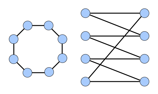
As you can see, the left-hand graph is much easier to interpret.

• Maximize the distance between unconnected nodes. If two unconnected nodes are placed near one another, the reader can be confused into thinking that they are somehow related when in fact there is no connection between them. For example, consider the two drawings below:

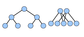
Again, the left-hand graph is much easier to interpret.

Algorithmically placing nodes according to these heuristics is difficult since the position of each node influences the position of each other node. Thus a direct approach requires solving a large, complex system of equations. However, there is an easier way for us…

Layout via Physics Simulation

Rather than solving for the answer directly, we’ll instead start with a random layout, then continuously refine the positions of the nodes to improve upon the heuristics. Over time, the nodes will reach a positions that balance the heuristics, and we’ll end up with an aesthetically pleasing graph drawing.

The key step in this algorithm is deciding how to update node positions, and to do this we’ll take a cue from physics. At each step of the graph layout, we’ll have the nodes exert forces on one another. These forces will push and pull nodes that are in sub-optimal positions until they eventually come to rest in a stable location. Because we want unconnected nodes to be far apart from one another, we’ll have each node repel each other node with some force. Similarly, because we want connected nodes to remain near one another, we’ll have each edge between nodes attract its endpoints. As these forces move the nodes around, the positions of the nodes will tend toward configurations where the net force on each node is minimized; that is, when there is a balance between the forces spacing out unconnected nodes and keeping together connected nodes.

The details of each step is customizable: we can initialize the positions of the nodes however we choose, decide when the layout is good enough to stop, and use almost any function to determine the strengths of the attractive and repulsive forces. We’ll outline one set of design choices below, but we encourage you to try out your own variations; I’ve suggested several ideas at the end of this handout.

1. Assigning initial node positions. There is no one “correct way” to initially lay out the nodes in the graph. Because the algorithm takes an initial guess and improves over time, pretty much any initial layout will do, but some initial layouts will enable faster convergance. You’ll initially position the nodes so that they are evenly spaced apart on the unit circle. In particular, in a graph with \(n\) nodes, the \(k^{th}\) node should be placed at

   \[ \left(\cos\frac{2 \pi k}{n},\sin\frac{2 \pi k}{n} \right)\]

   Here, angles are represented in radians.

2. Determining when we’re finished. If the algorithm stops too early, then the nodes may not have moved into good positions; if it runs too long, the computer will waste time trying to improve upon an already perfect layout. There are ways to automatically detect whether to continue (or simply run for a fixed duration), but we’ll just let the user decide when to stop.

3. Computing forces. The particular approach we will use to compute forces is based on the Fruchterman-Reingold algorithm. In Fruchterman-Reingold, every node exerts a repulsive force on every other node that is inversely proportional to the distance between those nodes, and each edge exerts an attractive force on its endpoints proportional to the square of the distance between those nodes. This means that as connected nodes grow more distant to one another, the attractive force rises quickly and the repulsive force drops off, so connected nodes will have a tendency to “snap back” toward one another. Similarly, as the nodes draw increasingly close, the repulsive force grows rapidly while the attractive force diminishes, so the nodes will move away from each other. Only when the nodes are at a perfect distance from one another will the forces balance and the nodes cease to move.

   To keep track of the net forces on each node \(a\), you’ll maintain \(\Delta x_a\) and \(\Delta y_a\) values storing the net forces on node \(a\) along the x and y axes. The net forces in each direction begin at zero, but will be adjusted by the interactions of each node with each other node:

   Initial Forces

   For each node \(a\) at \((x_a, y_a)\):

   • \(\Delta x_a = 0\)
   • \(\Delta y_a = 0\)

   The first source of force acting on each node is the repulsive force exerted by every node against every other node. For each pair of nodes \(a\) and \(b\) at positions \((x_a, y_a)\) and \((x_b, y_b)\), the magnitude of the repulsive force F_{repel} between these nodes is

   \[ F_{repel} = \frac{k_{repel}}{\sqrt{ (x_b - x_a)^2 + (y_b - y_a)^2 }} \]

   Where \(k_repel\) is a constant that controls the strength of the repulsive attraction. If the magnitude of this constant increases, then nodes repel each other more strongly; if it has a small magnitude, then nodes hardly repel each other at all. A value of \(0.005\) will work to get started, but you are free to experiment with this value if you wish.

   Once you have computed the magnitude of the repulsive force, you will need to determine how much of that force is in the y-direction and how much of it is in the x-direction. To see how this force splits up, consider the following diagram:

   

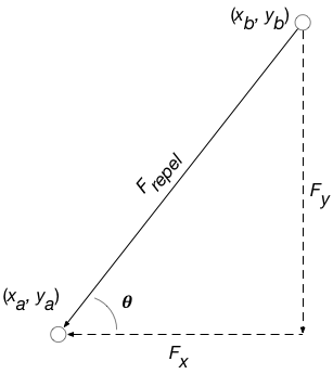
   Here, \(F_x\) and \(F_y\) are the forces in the x and y directions exerted on the node at \((x_a, y_a)\). Using some simple trigonometry, we get that

   \[ \begin{array}{rcl} F_{x_a} & = & −F_{repel} \cdot \cos \theta \\ F_{y_a} & = & −F_{repel} \cdot \sin \theta \end{array} \]

   By Newton’s laws, the force exerted against the node \((x_b, y_b)\) are the opposite:

   \[ \begin{array}{rcl} F_{x_b} & = & F_{repel} \cdot \cos \theta \\ F_{y_b} & = & F_{repel} \cdot \sin \theta \end{array} \]

   Here, we’ve been using the angle \(\theta\) to represent the angle indicated in the above drawing. Again, simple trigonometry tells us that

   \[ \theta = \tan^{-1} \frac{y_b - y_a}{x_b - x_a} \]

   To summarize, the algorithm for computing repulsive forces is as follows:

   Computing Repulsive Forces

   For each pair of nodes \(a\) and \(b\) at locations \((x_a, y_a)\) and \((x_b, y_b)\), respectively:

   • Compute force and angle between nodes:
     • \(F_{repel} = \frac{k_{repel}}{\sqrt{ (x_b - x_a)^2 + (y_b - y_a)^2 }}\)
     • \(\theta = \tan^{-1} \frac{y_b - y_a}{x_b - x_a}\)
   • Update forces on each node:
     • \(\Delta x_a\) -= \(F_{repel} \cdot \cos \theta\)
     • \(\Delta y_a\) -= \(F_{repel} \cdot \sin \theta\)
     • \(\Delta x_b\) += \(F_{repel} \cdot \cos \theta\)
     • \(\Delta y_b\) += \(F_{repel} \cdot \sin \theta\)

   The second source of force acting on each node is the attractive forces between nodes joined together by edges. In this case, the attractive force \(F_{attract}\) is proportional to the square of the distance between the nodes:

   \[ F_{attract} = {k_{attract}} \cdot ((x_b - x_a)^2 + (y_b - y_a)^2) \]

   As above, \(k_{attract}\) is a constant controlling the strength of the attractive force and using the value \(0.005\) is a good starting point. Following similar reasoning as for repulsive forces, we can compute how this force divides over the x and y components as follows:
   Computing Attractive Forces

   For each edge from a node \(a\) at \((x_a, y_a)\) to a node \(b\) at \((x_b, y_b)\):

   • Compute force and angle between nodes:
     • \(F_{attract} = {k_{attract}} \cdot ((x_b - x_a)^2 + (y_b - y_a)^2))\)
     • \(\theta = \tan^{-1} \frac{y_b - y_a}{x_b - x_a}\)
   • Update forces on each node:
     • \(\Delta x_a\) += \(F_{attract} \cdot \cos \theta\) // Note that this is +=, not -=!
     • \(\Delta y_a\) += \(F_{attract} \cdot \sin \theta\)
     • \(\Delta x_b\) -= \(F_{attract} \cdot \cos \theta\) // Note that this is -=, not +=!
     • \(\Delta y_b\) -= \(F_{attract} \cdot \sin \theta\)

    

4. Moving Nodes According to the Forces. Once you’ve computed the net \(\Delta x_a\) and \(\Delta y_a\) forces for each node \(a\), moving the nodes is easy:

   Moving Nodes

   For each node \(a\) at \((x_a, y_a)\):

   • Move \(a\) to \((x_a + \Delta x_a, y_a + \Delta y_a)\)

   (Note that in a true physical simulation the forces on each object would change the velocity of the object rather than directly modifying its position, but changing positions is sufficient. If you’d like to experiment with each node having a velocity and a position, feel free to do so.)