Midterm Review Session
Midterm Review Session#
This is the code we wrote during the review session.
# Run this cell to set up the notebook.
# These lines import the numpy, datascience, and cs104 libraries.

import numpy as np
from datascience import *
from cs104 import *
%matplotlib inline
Here’s a loop that inspects the contents of an array and does something to each element:
for word in make_array("Cow", "Goat", "Dog"):
    print(word)
Cow
Goat
Dog
Here’s a loop that does “something” a specific number of times (also known as a counting loop):
dice = np.arange(1,7)
for i in np.arange(0,5):
    print(np.random.choice(dice))
4
6
5
1
5
Here’s a loop that inspects elements of an array and counts the number elements that meet some criteria. In this case, we are counting the positive numbers:
def stay_positive(values):
    count = 0
    for i in values:
        if i > 0:
            count = count + 1
    return count
This is a version of the same function that uses array broadcasting and np.count_nonzero:
stay_positive(make_array(1,-1,-2,3,4,0))
def stay_positive(values):
    return np.count_nonzero(values > 0)

stay_positive(make_array(1,-1,-2,3,4,0))
3
Here is a simple simulation loop that rolls 100 dice and counts the number of times we see a 6. We look at one outcome at a time and tally the outcomes matching our criteria:
dice = np.arange(1,7)
count = 0
for i in np.arange(0, 100):
    if np.random.choice(dice) == 6:
        count = count + 1

count
21
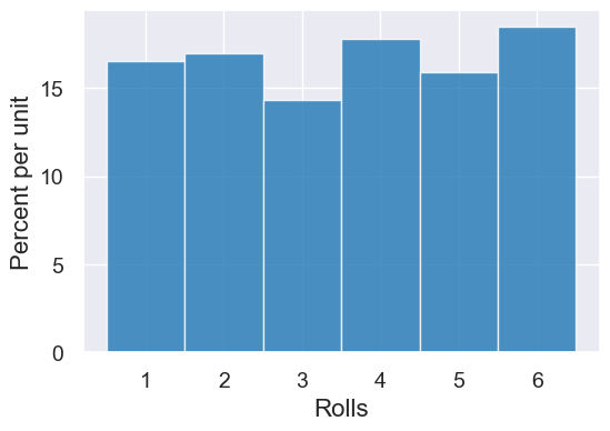
Here is a simple simulation loop that collects the outcomes of 1000 dice rolls in an array. That way, we can look at all outcomes after the simulation and, for example, plot a histogram:
dice = np.arange(1,7)
result = make_array()
for i in np.arange(0, 1000):
    roll = np.random.choice(dice)
    result = np.append(result, roll)

Table().with_columns("Rolls", result).hist(bins=np.arange(0.5,7.5,1))
Here are some apply examples:
finches = Table().read_table('data/finch_beaks_1975.csv')
finches.show(3)
| species | Beak length, mm | Beak depth, mm |
|---|---|---|
| fortis | 9.4 | 8 |
| fortis | 9.2 | 8.3 |
| scandens | 13.9 | 8.4 |
... (403 rows omitted)
Let’s add a new column that is the Beak length in inches.
def to_inch(mm):
    return mm / 25.4
to_inch(10)
0.3937007874015748
inches = finches.apply(to_inch, 'Beak length, mm')
new_finches = finches.with_columns('Beak Length, in', inches)
new_finches
| species | Beak length, mm | Beak depth, mm | Beak Length, in |
|---|---|---|---|
| fortis | 9.4 | 8 | 0.370079 |
| fortis | 9.2 | 8.3 | 0.362205 |
| scandens | 13.9 | 8.4 | 0.547244 |
| scandens | 14 | 8.8 | 0.551181 |
| scandens | 12.9 | 8.4 | 0.507874 |
| fortis | 9.5 | 7.5 | 0.374016 |
| fortis | 9.5 | 8 | 0.374016 |
| fortis | 11.5 | 9.9 | 0.452756 |
| fortis | 11.1 | 8.6 | 0.437008 |
| fortis | 9.9 | 8.4 | 0.389764 |
... (396 rows omitted)
Let’s compute a “beak area” too. (Okay, this is stretching credulity a bit, but it lets us demonstrate using apply with a function of two arguments.
def area(depth, length):
    return depth * length
areas = finches.apply(area, 'Beak depth, mm', 'Beak length, mm')
areas
array([ 75.2   ,  76.36  , 116.76  , 123.2   , 108.36  ,  71.25  ,
        76.    , 113.85  ,  95.46  ,  83.16  , 112.7   ,  99.36  ,
       101.7   , 109.25  , 102.35  ,  85.36  , 105.73  , 107.365 ,
        89.89  ,  90.1   ,  78.72  ,  95.79  ,  95.55  ,  92.4   ,
       102.46  , 107.52  ,  79.9   ,  81.81  ,  76.8   , 101.85  ,
        81.18  ,  83.16  ,  75.84  ,  99.51  , 123.9   ,  98.94  ,
       104.64  ,  71.61  , 113.68  , 109.76  ,  85.85  ,  98.44  ,
       111.1   ,  97.2   ,  91.8   , 101.52  ,  91.52  , 110.88  ,
       112.86  ,  97.01  ,  97.76  ,  79.54  ,  83.64  ,  74.52  ,
        84.84  , 111.1   ,  88.58  ,  86.7   , 106.7   , 113.3   ,
        86.86  ,  99.51  ,  95.23  , 106.7   , 122.4   , 118.32  ,
        84.15  ,  95.04  ,  93.45  ,  87.    ,  89.28  , 106.7   ,
        97.92  ,  76.145 , 106.56  ,  96.72  , 108.78  ,  89.76  ,
        93.73  ,  89.1   , 114.4   ,  97.2   ,  99.75  ,  91.35  ,
       107.52  , 105.28  , 111.15  ,  90.3   , 103.95  , 105.28  ,
        91.    ,  89.44  , 100.44  , 102.12  ,  90.64  , 102.12  ,
        81.34  ,  92.4   , 103.4   , 116.48  ,  83.3   ,  77.42  ,
        77.42  , 104.03  , 110.74  ,  83.    , 104.34  ,  90.    ,
        86.52  ,  88.74  ,  95.68  , 104.5   , 116.15  , 115.64  ,
        86.7   , 119.34  ,  86.86  ,  94.86  ,  85.26  ,  94.34  ,
        84.    , 124.63  , 109.89  ,  93.45  ,  91.    ,  87.72  ,
        75.66  ,  86.    , 101.65  , 104.5   , 111.18  ,  95.55  ,
       105.73  , 100.58  , 124.95  ,  91.8   , 102.9   , 112.    ,
       102.72  ,  98.88  , 114.84  ,  97.65  , 104.64  ,  74.48  ,
       100.28  ,  90.64  , 118.17  ,  97.9   ,  93.1   ,  85.28  ,
       104.76  , 107.8   ,  98.58  , 110.74  ,  88.88  , 115.14  ,
       123.9   ,  85.14  , 106.7   , 108.    , 109.61  , 116.55  ,
       114.4   ,  95.68  ,  73.71  , 101.52  ,  94.34  ,  71.34  ,
        99.51  ,  88.58  ,  94.5   ,  69.16  ,  82.65  , 105.84  ,
        99.64  ,  98.01  , 116.15  , 109.76  ,  76.63  , 131.76  ,
        72.68  , 105.    ,  88.2   , 102.6   ,  94.16  , 122.72  ,
        73.71  ,  98.98  ,  82.    , 104.5   , 128.1   , 110.58  ,
       104.64  , 101.76  ,  73.47  , 110.09  ,  98.58  , 113.3   ,
        71.1   , 100.1   ,  92.56  ,  86.32  ,  90.24  , 100.7   ,
        85.85  ,  83.42  ,  81.6   ,  82.82  ,  78.21  , 110.    ,
       102.46  ,  77.6   ,  86.    ,  93.6   , 114.84  ,  76.8   ,
       103.68  , 100.28  ,  91.8   ,  91.8   ,  95.68  , 104.5   ,
        98.44  , 107.67  ,  98.28  , 102.46  ,  85.14  , 115.64  ,
        77.6   , 123.76  ,  77.76  , 107.91  ,  87.72  ,  79.2   ,
       101.7   , 105.73  ,  79.38  ,  90.64  ,  66.    , 118.32  ,
        81.18  ,  85.14  ,  86.13  ,  89.44  , 110.88  , 102.6   ,
        83.16  ,  86.13  ,  83.64  ,  95.68  ,  77.08  ,  93.84  ,
       102.3   ,  94.34  ,  94.5   ,  94.64  ,  89.76  ,  89.76  ,
       105.6   , 113.22  ,  79.54  ,  93.45  ,  98.1   ,  94.16  ,
       108.9   , 101.37  , 110.88  , 109.25  , 108.    ,  90.78  ,
       107.8   , 107.91  ,  91.35  ,  99.36  ,  80.36  ,  76.63  ,
        93.73  ,  85.49  ,  85.49  , 125.28  , 125.28  , 107.91  ,
        95.4   , 106.95  , 103.68  , 100.719 , 119.646 ,  87.978 ,
       129.8934, 117.5004, 103.008 ,  95.8624,  97.185 , 108.382 ,
       100.9245, 114.954 ,  98.4555,  84.405 , 117.915 ,  83.555 ,
        80.0253, 104.94  , 123.0768, 113.3884,  95.497 ,  88.131 ,
        92.8725, 112.2975,  96.9075,  84.2175,  91.7375, 126.3125,
       110.0475, 111.1425,  89.1475,  85.4025, 117.3625,  99.9375,
        89.9475, 116.76  , 123.2   , 108.36  , 108.    , 101.91  ,
       129.94  , 111.8   , 120.7   , 124.6   , 129.22  , 112.66  ,
       147.98  , 110.7   , 129.6   , 144.53  , 110.94  , 106.6   ,
       134.1   , 117.6   , 118.68  , 115.7   , 134.225 , 113.71  ,
       120.06  , 134.4   , 124.1   , 138.32  , 121.5   , 138.92  ,
       148.5   , 110.08  , 137.08  , 128.52  , 119.26  , 120.7   ,
       157.04  , 144.96  , 127.4   , 126.48  , 130.2   , 123.2   ,
       115.37  , 123.2   , 135.59  , 157.56  , 122.82  , 132.48  ,
       108.8   , 144.84  , 135.34  , 128.8   , 143.56  , 129.22  ,
       114.75  , 109.88  , 131.4   , 125.55  , 109.6   , 126.49  ,
       106.11  , 111.22  , 120.06  , 119.68  , 120.4   , 117.45  ,
       102.4   , 123.2   , 120.6   , 135.59  , 151.3596, 133.133 ,
       144.354 , 163.592 , 123.089 , 150.4736, 136.8656, 128.07  ,
       128.0575, 138.4775, 141.2775, 120.6675, 132.7725, 137.4975,
       127.1525, 126.4375, 142.2225, 110.6375])
finches_with_area = finches.with_columns('Beak area, mm^2', areas)
finches_with_area.show(3)
| species | Beak length, mm | Beak depth, mm | Beak area, mm^2 |
|---|---|---|---|
| fortis | 9.4 | 8 | 75.2 |
| fortis | 9.2 | 8.3 | 76.36 |
| scandens | 13.9 | 8.4 | 116.76 |
... (403 rows omitted)
Overlaid histograms enable us to divide rows of a table into groups that are displayed separately. Compare this histogram:
finches.hist('Beak length, mm')
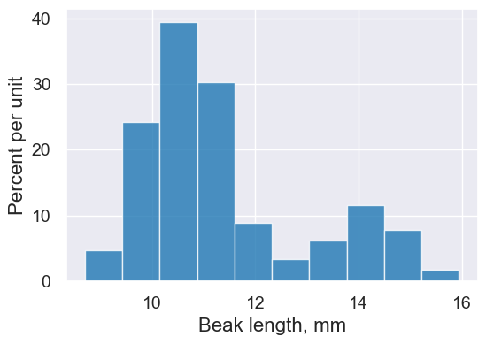
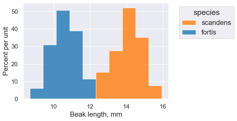
to this one, where we group our observations by species. It lets us identify the characteristics of our different groups much more easily.
finches.hist('Beak length, mm', group='species')
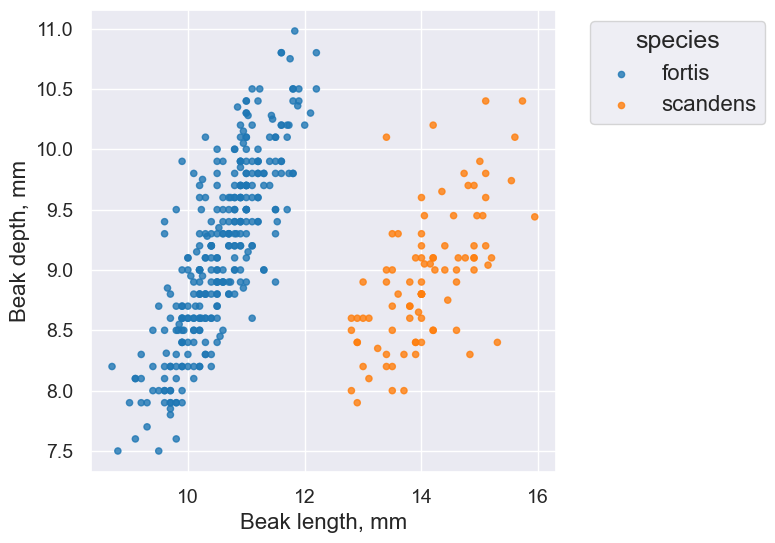
One last example:
finches.scatter('Beak length, mm', 'Beak depth, mm', group='species')