Randomized Controlled Experiments
Contents
Randomized Controlled Experiments#
from datascience import *
from cs104 import *
import numpy as np
%matplotlib inline
1. Warm-up Permutation Test#
survey = Table().read_table('data/prelab01-survey-fall2023.csv')
survey = survey.where('Left or Right Handed', are.not_equal_to('Ambidextrous'))
survey
| Year at Williams | Favorite Icecream Flavor | Favorite Planet | Height (in inches) | Distance Home (in miles) | Birth Month | Left or Right Handed |
|---|---|---|---|---|---|---|
| 2 | Strawberry | Venus | 60 | 175 | October | Right |
| 1 | Coffee | Venus | 63 | 6831 | March | Right |
| 2 | Chocolate | Earth | 74 | 2600 | July | Right |
| 1 | Chocolate | Saturn | 64 | 141 | July | Right |
| 1 | Chocolate | Earth | 66 | 132.8 | October | Right |
| 1 | I don't like icecream! | Earth | 73 | 2023 | October | Right |
| 2 | Vanilla | Saturn | 66 | 1685.7 | June | Right |
| 2 | Chocolate | Pluto | 69 | 167.5 | April | Right |
| 2 | Chocolate | Jupiter | 62 | 170 | December | Right |
| 4 | Vanilla | Earth | 71 | 7233 | January | Right |
... (47 rows omitted)
survey.group('Left or Right Handed', np.mean)
| Left or Right Handed | Year at Williams mean | Favorite Icecream Flavor mean | Favorite Planet mean | Height (in inches) mean | Distance Home (in miles) mean | Birth Month mean |
|---|---|---|---|---|---|---|
| Left | 2.8 | 69.6 | 1419.4 | |||
| Right | 2.30769 | 68.6362 | 1295.68 |
observed = abs_difference_of_means(survey, 'Left or Right Handed', 'Height (in inches)')
observed
0.9638461538461485
Is the height difference significant?
results = simulate_permutation_statistic(survey, 'Left or Right Handed', 'Height (in inches)', 1000)
plot = Table().with_columns('abs_difference_of_means', results).hist(left_end=observed)
plot.set_title('Null hypothesis empirical distibution')
plot.dot(observed)
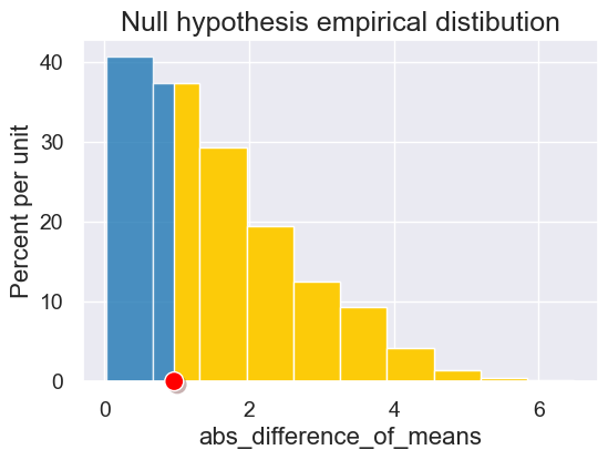
p_value = empirical_pvalue(results, observed)
p_value
0.653
2. Randomized Controlled Experiment with BTA#
rct = Table.read_table('data/bta.csv')
rct.sample(10)
| Group | Result |
|---|---|
| Control | 0 |
| Treatment | 1 |
| Control | 0 |
| Treatment | 1 |
| Treatment | 1 |
| Treatment | 0 |
| Treatment | 1 |
| Control | 0 |
| Control | 0 |
| Treatment | 1 |
rct.group('Group')
| Group | count |
|---|---|
| Control | 16 |
| Treatment | 15 |
rct.pivot('Result', 'Group')
| Group | 0.0 | 1.0 |
|---|---|---|
| Control | 14 | 2 |
| Treatment | 6 | 9 |
rct.group('Group', np.mean)
| Group | Result mean |
|---|---|
| Control | 0.125 |
| Treatment | 0.6 |
Permutation Testing#
observed_statistic = abs_difference_of_means(rct, 'Group', 'Result')
observed_statistic
0.475
type(observed_statistic)
float
results = simulate_permutation_statistic(rct, 'Group', 'Result', 2000)
plot = Table().with_columns('Abs Difference in Relief Proportions', results).hist(bins=np.arange(0,0.9,1/16))
plot.set_title('Null hypothesis empirical distibution')
plot.dot(observed_statistic)
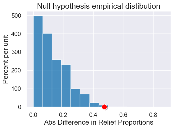
p_value = empirical_pvalue(results, observed_statistic)
p_value
0.009
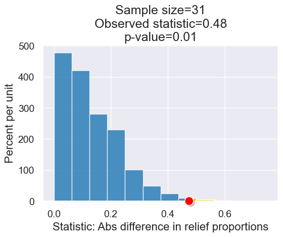
3. Sample Size, Effect Size, and P-values#
What’s the relationship between effect size, sample size, and p-value?
What we had before.
What if the effect size was slightly smaller? What if the sample size was bigger?
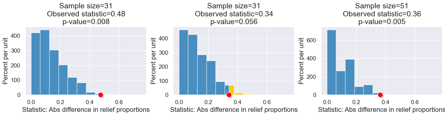
Let’s look at all these relationships at once!
The following cell contains an interactive visualization. You won’t see the visualization on this web page, but you can view and interact with it if you run this notebook on our server here.
interact(back_pain_exploration,
         observed_sample_size=Slider(10, 200, 1),
         treatment_prop_effective=Slider(0.05, 0.95, 0.01),
         control_prop_effective=Slider(0.05, 0.95, 0.01))
Here’s an animation showing the effects above.