Wrap Up
1. Installing Python packages
Install packages in a Jupyter notebook on any machine (including your own)!
# Three packages we have used throughout the semester
!pip3 install -q datascience
!pip3 install -q numpy
!pip3 install -q matplotlib
We import packages that have been installed in order to use their features in our code:
# Second step: import packages
from datascience import *
import numpy as np
import matplotlib.pyplot as plots
%matplotlib inline
Now let’s install three different packages we haven’t seen yet…
!pip3 install -q pandas
!pip3 install -q scikit-learn
!pip3 install -q seaborn
import pandas as pd
from sklearn import *
import seaborn as sns
2. Pandas
Pandas is a library to manipulate and explore data (similar to Tables), but with more functionality.
penguins = pd.read_csv('https://raw.githubusercontent.com/mcnakhaee/palmerpenguins/master/palmerpenguins/data/penguins.csv')
penguins = penguins.drop(columns = ['year'])
penguins.head(6)
| species | island | bill_length_mm | bill_depth_mm | flipper_length_mm | body_mass_g | sex | |
|---|---|---|---|---|---|---|---|
| 0 | Adelie | Torgersen | 39.1 | 18.7 | 181.0 | 3750.0 | male |
| 1 | Adelie | Torgersen | 39.5 | 17.4 | 186.0 | 3800.0 | female |
| 2 | Adelie | Torgersen | 40.3 | 18.0 | 195.0 | 3250.0 | female |
| 3 | Adelie | Torgersen | NaN | NaN | NaN | NaN | NaN |
| 4 | Adelie | Torgersen | 36.7 | 19.3 | 193.0 | 3450.0 | female |
| 5 | Adelie | Torgersen | 39.3 | 20.6 | 190.0 | 3650.0 | male |
# pandas gives us a quick summary of the data
penguins.info()
<class 'pandas.core.frame.DataFrame'>
RangeIndex: 344 entries, 0 to 343
Data columns (total 7 columns):
 #   Column             Non-Null Count  Dtype
---  ------             --------------  -----
 0   species            344 non-null    object
 1   island             344 non-null    object
 2   bill_length_mm     342 non-null    float64
 3   bill_depth_mm      342 non-null    float64
 4   flipper_length_mm  342 non-null    float64
 5   body_mass_g        342 non-null    float64
 6   sex                333 non-null    object
dtypes: float64(4), object(3)
memory usage: 18.9+ KB
penguins = penguins.dropna()
penguins.head(6)
| species | island | bill_length_mm | bill_depth_mm | flipper_length_mm | body_mass_g | sex | |
|---|---|---|---|---|---|---|---|
| 0 | Adelie | Torgersen | 39.1 | 18.7 | 181.0 | 3750.0 | male |
| 1 | Adelie | Torgersen | 39.5 | 17.4 | 186.0 | 3800.0 | female |
| 2 | Adelie | Torgersen | 40.3 | 18.0 | 195.0 | 3250.0 | female |
| 4 | Adelie | Torgersen | 36.7 | 19.3 | 193.0 | 3450.0 | female |
| 5 | Adelie | Torgersen | 39.3 | 20.6 | 190.0 | 3650.0 | male |
| 6 | Adelie | Torgersen | 38.9 | 17.8 | 181.0 | 3625.0 | female |
print('num rows (after droping nulls) = ', len(penguins))
num rows (after droping nulls) = 333
penguins[penguins.species == 'Adelie'].mean(numeric_only=True)
bill_length_mm         38.823973
bill_depth_mm          18.347260
flipper_length_mm     190.102740
body_mass_g          3706.164384
dtype: float64
3. Seaborn
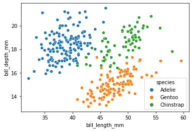
Seaborn is a Data visualization library. Interfaces with pandas nicely. Makes very pretty plots!
sns.scatterplot(penguins, x="bill_length_mm", y="bill_depth_mm", hue="species");
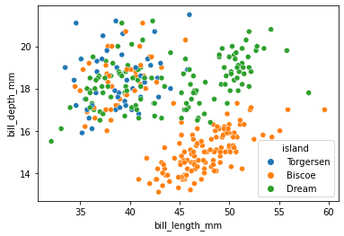
A big advantage of seaborn is that you can quickly visualize different subsets of data:
sns.scatterplot(penguins, x="bill_length_mm", y="bill_depth_mm", hue="island");
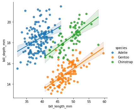
sns.lmplot(penguins, x="bill_length_mm", y="bill_depth_mm", hue="species");
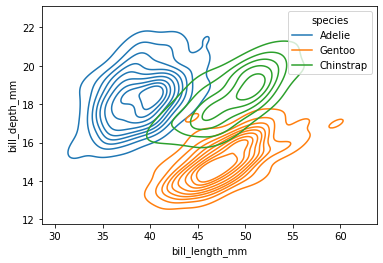
sns.kdeplot(penguins, x="bill_length_mm", y="bill_depth_mm", hue="species");
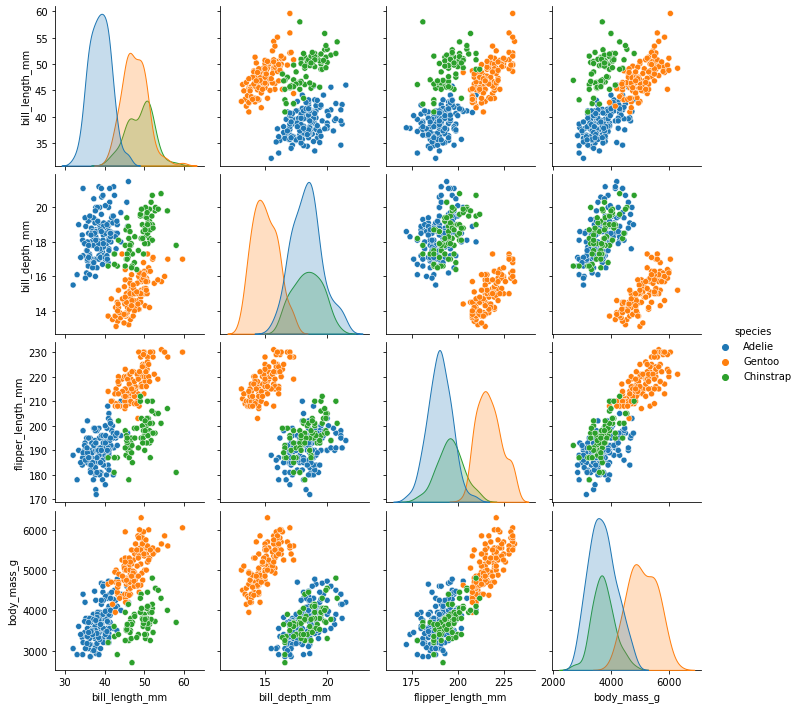
sns.pairplot(penguins, hue="species");
fig, ax = plots.subplots(1,2,figsize=(12,5))
sns.scatterplot(penguins, x="bill_length_mm", y="bill_depth_mm", hue="species",
                size="body_mass_g", sizes=(30, 300), alpha=0.5,
                ax=ax[0])
sns.violinplot(penguins, x="body_mass_g", y="species", hue="sex",
               ax=ax[1])
fig.tight_layout();

4. sklearn (Scikit-Learn)
sklearn — pronounced Sci Kit Learn — is a library for machine learning (statistical pattern matching).
Linear Regression with sklearn
from sklearn import linear_model

from sklearn.metrics import r2_score as r2_score_sklearn
from sklearn.metrics import mean_squared_error as mse_sklearn
from sklearn.feature_selection import r_regression
# Some data wrangling to get our x and y values, this time with pandas...
chinstrap = penguins[penguins['species'] == 'Chinstrap']
x = chinstrap['bill_length_mm'].to_numpy().reshape(-1, 1)
y = chinstrap['bill_depth_mm'].to_numpy()
model = linear_model.LinearRegression()
model.fit(x, y);
print('slope    ', model.coef_[0])
print('intercept', model.intercept_)
slope     0.2222117240036715
intercept 7.569140119132472
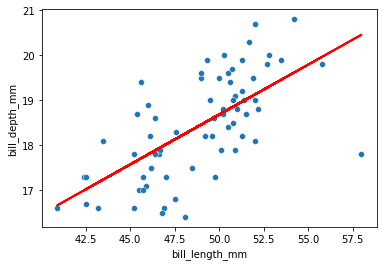
y_hat = model.predict(x)
sns.scatterplot(chinstrap, x='bill_length_mm', y='bill_depth_mm')
plots.plot(x, y_hat, color='r', lw=2);
A whole lot of metrics we might want are already implemented in sklearn.
print('Pearson Correlation:', r_regression(x, y)[0])
print('MSE:                ', mse_sklearn(y, y_hat))
print('R2 Score:           ', r2_score_sklearn(y, y_hat))
Pearson Correlation: 0.6535362081800236
MSE:                 0.7276649994299124
R2 Score:            0.4271095754023476
Non-linear Regresion
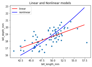
New: let’s fit a non-linear regression line with sklearn!
model_nonlinear = svm.SVR(kernel='poly') #does non-linear (polynomial) regression
model_nonlinear.fit(x, y);
# plot what the polynomial regression does
x_range = np.arange(42.5, 57.5, 0.1).reshape(-1, 1)

y_hat_linear = model.predict(x_range)
y_hat_nonlinear = model_nonlinear.predict(x_range)

sns.scatterplot(chinstrap, x='bill_length_mm', y='bill_depth_mm')
plots.plot(x_range, y_hat_linear, color='r', label='linear', lw=2);
plots.plot(x_range, y_hat_nonlinear, color='b', label='nonlinear', lw=2)
plots.title("Linear and Nonlinear models")
plots.legend();
Take Machine Learning to learn the process for evaluating which model is better!