Correlation
from datascience import *
%matplotlib inline
import matplotlib.pyplot as plots
plots.style.use('fivethirtyeight')
import numpy as np
import warnings
warnings.simplefilter(action='ignore', category=np.VisibleDeprecationWarning)
warnings.simplefilter(action='ignore', category=UserWarning)

from ipywidgets import interact, interactive, fixed, interact_manual, FloatSlider
import ipywidgets as widgets
Hypothesis Testing with Confidence Intervals: Biased Coin?
Observed sample: 45 heads, 55 tails
Null Hypothesis: Coin is not biased, so expect 50% chance of heads on each flip
Alt Hypothesis: Coin is biased
observed_sample_size = 100
observed_num_heads = 45

observed_sample = Table().with_columns('flips',
                                       np.append(np.full(observed_num_heads, 'heads'),
                                                 np.full(observed_sample_size - observed_num_heads, 'tails')))
observed_sample.column('flips')
array(['heads', 'heads', 'heads', 'heads', 'heads', 'heads', 'heads',
       'heads', 'heads', 'heads', 'heads', 'heads', 'heads', 'heads',
       'heads', 'heads', 'heads', 'heads', 'heads', 'heads', 'heads',
       'heads', 'heads', 'heads', 'heads', 'heads', 'heads', 'heads',
       'heads', 'heads', 'heads', 'heads', 'heads', 'heads', 'heads',
       'heads', 'heads', 'heads', 'heads', 'heads', 'heads', 'heads',
       'heads', 'heads', 'heads', 'tails', 'tails', 'tails', 'tails',
       'tails', 'tails', 'tails', 'tails', 'tails', 'tails', 'tails',
       'tails', 'tails', 'tails', 'tails', 'tails', 'tails', 'tails',
       'tails', 'tails', 'tails', 'tails', 'tails', 'tails', 'tails',
       'tails', 'tails', 'tails', 'tails', 'tails', 'tails', 'tails',
       'tails', 'tails', 'tails', 'tails', 'tails', 'tails', 'tails',
       'tails', 'tails', 'tails', 'tails', 'tails', 'tails', 'tails',
       'tails', 'tails', 'tails', 'tails', 'tails', 'tails', 'tails',
       'tails', 'tails'], dtype='<U5')
def percent_heads(sample):
    return 100 * sum(sample.column('flips') == 'heads') / sample.num_rows

percent_heads(observed_sample)
45.0
def bootstrap(observed_sample, num_trials):

    bootstrap_statistics = make_array()

    for i in np.arange(0, num_trials):

        simulated_resample = observed_sample.sample()
        resample_statistic = percent_heads(simulated_resample)

        bootstrap_statistics = np.append(bootstrap_statistics, resample_statistic)

    return bootstrap_statistics
def percentile_method(ci_percent, bootstrap_statistics):
    """
    Return an array with the lower and upper bound of the ci_percent confidence interval.
    """
    # percent in each of the the left/right tails
    percent_in_each_tail = (100 - ci_percent) / 2
    left = percentile(percent_in_each_tail, bootstrap_statistics)
    right = percentile(100 - percent_in_each_tail, bootstrap_statistics)
    return make_array(left, right)
bootstrap_statistics = bootstrap(observed_sample, 1000)
results = Table().with_columns("Percent Heads", bootstrap_statistics)
results.hist()
plots.scatter(percent_heads(observed_sample), 0, color='red', s=100, zorder=10, clip_on=False);
left_right = percentile_method(95, bootstrap_statistics)
plots.plot(left_right, [0, 0], color='yellow', lw=8);
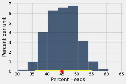
“50% heads” (Null Hypothesis) is in the 95% confidence interval, so we cannot reject the Null Hypothesis.
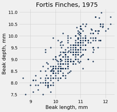
Finch data and visualizations
# Load finch data
finch_1975 = Table().read_table("data/finch_beaks_1975.csv")
finch_1975.show(6)
| species | Beak length, mm | Beak depth, mm |
|---|---|---|
| fortis | 9.4 | 8 |
| fortis | 9.2 | 8.3 |
| scandens | 13.9 | 8.4 |
| scandens | 14 | 8.8 |
| scandens | 12.9 | 8.4 |
| fortis | 9.5 | 7.5 |
... (400 rows omitted)
fortis = finch_1975.where('species', 'fortis')
fortis.num_rows
316
scandens = finch_1975.where('species', 'scandens')
scandens.num_rows
90
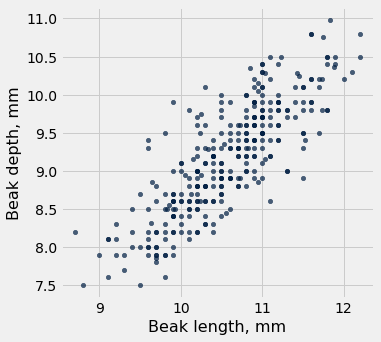
fortis.scatter('Beak length, mm', 'Beak depth, mm')
plots.title('Fortis Finches, 1975');
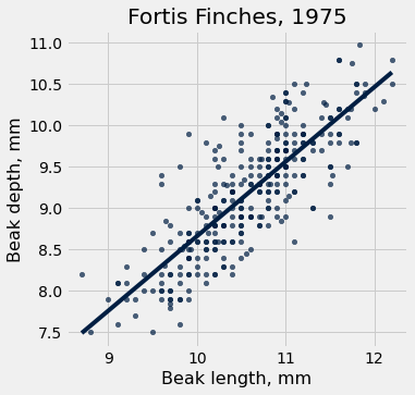
fortis.scatter('Beak length, mm', 'Beak depth, mm', fit_line=True)
plots.title('Fortis Finches, 1975');
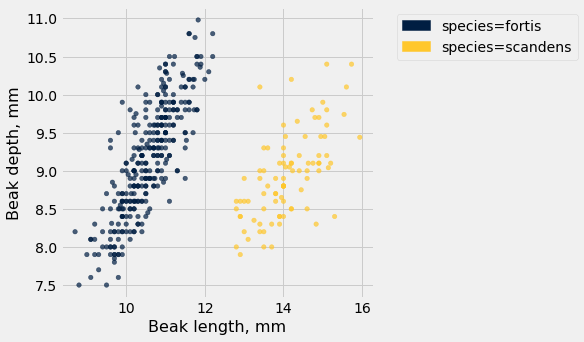
finch_1975.scatter('Beak length, mm', 'Beak depth, mm', group='species')
Correlation
Visualize different values of r:
def r_scatter(r):
    plots.figure(figsize=(5,5))
    "Generate a scatter plot with a correlation approximately r"
    x = np.random.normal(0, 1, 1000)
    z = np.random.normal(0, 1, 1000)
    y = r*x + (np.sqrt(1-r**2))*z
    plots.scatter(x, y,s=20)
    plots.xlim(-4, 4)
    plots.ylim(-4, 4)
    plots.title('r='+str(r));

_ = widgets.interact(r_scatter,
                     r = (-1,1,0.01));
Computing Pearson’s Correlation Coefficient
The formula: \( r = \frac{\sum(x - \bar{x})(y - \bar{y})}{\sqrt{\sum(x - \bar{x})^2} \sqrt{\sum(y - \bar{y})^2}} \)
def pearson_correlation(table, x_label, y_label):
    x = table.column(x_label)
    y = table.column(y_label)
    x_mean = np.mean(x)
    y_mean = np.mean(y)
    numerator = sum((x - x_mean) * (y - y_mean))
    denominator = np.sqrt(sum((x - x_mean)**2)) * np.sqrt(sum((y - y_mean)**2))
    return numerator / denominator
fortis_r = pearson_correlation(fortis, 'Beak length, mm', 'Beak depth, mm')
fortis_r
0.8212303385631524
scandens_r = pearson_correlation(scandens, 'Beak length, mm', 'Beak depth, mm')
scandens_r
0.624688975610796
CIs for Correlation coefficient via bootstrapping
def bootstrap_finches(observed_sample, num_trials):

    bootstrap_statistics = make_array()

    for i in np.arange(0, num_trials):

        simulated_resample = observed_sample.sample()

        # this changes for this example
        resample_statistic = pearson_correlation(simulated_resample, 'Beak length, mm', 'Beak depth, mm')

        bootstrap_statistics = np.append(bootstrap_statistics, resample_statistic)

    return bootstrap_statistics
fortis_bootstraps = bootstrap_finches(fortis, 10000)
scandens_bootstraps = bootstrap_finches(scandens, 10000)
fortis_ci = percentile_method(95, fortis_bootstraps)
print('Fortis r = ', fortis_r)
print('Fortis CI=', fortis_ci)
Fortis r =  0.8212303385631524
Fortis CI= [0.78179936 0.85502018]
scandens_ci = percentile_method(95, scandens_bootstraps)
print('Scandens r = ', scandens_r)
print('Scandens CI=', scandens_ci)
Scandens r =  0.624688975610796
Scandens CI= [0.46836757 0.75198562]
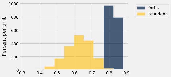
Table().with_columns('fortis', fortis_bootstraps, 'scandens', scandens_bootstraps).hist()
Switching Axes
fortis.scatter('Beak length, mm', 'Beak depth, mm')
pearson_correlation(fortis, 'Beak length, mm', 'Beak depth, mm')
0.8212303385631524
fortis.scatter('Beak depth, mm','Beak length, mm')
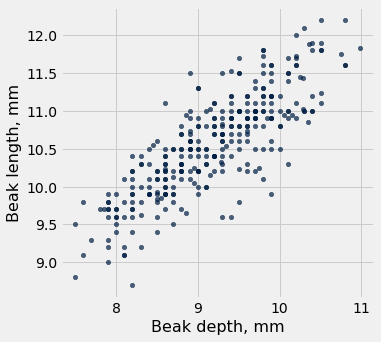
pearson_correlation(fortis, 'Beak depth, mm', 'Beak length, mm')
0.8212303385631524
Watch out for…
Nonlinearity
new_x = np.arange(-4, 4.1, 0.5)
nonlinear = Table().with_columns(
        'x', new_x,
        'y', new_x**2
    )
nonlinear.scatter('x', 'y', s=50, color='red')
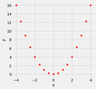
pearson_correlation(nonlinear, 'x', 'y')
0.0
Outliers
What can cause outliers? What to do when you encounter them?
line = Table().with_columns(
        'x', make_array(1, 2, 3, 4),
        'y', make_array(1, 2, 3, 4)
    )
line.scatter('x', 'y', s=50, color='red')
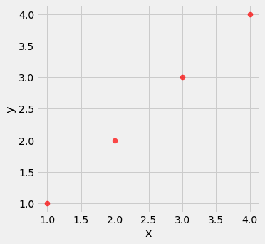
pearson_correlation(line, 'x', 'y')
0.9999999999999998
outlier = Table().with_columns(
        'x', make_array(1, 2, 3, 4, 5),
        'y', make_array(1, 2, 3, 4, 0)
    )
outlier.scatter('x', 'y', s=50, color='red')
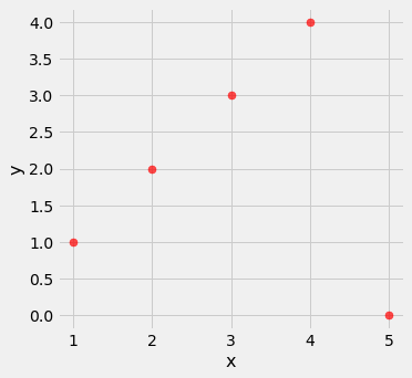
pearson_correlation(outlier, 'x', 'y')
0.0
False Correlations due to Data Aggregation
sat2014 = Table.read_table('data/sat2014.csv').sort('State')
sat2014
| State | Participation Rate | Critical Reading | Math | Writing | Combined |
|---|---|---|---|---|---|
| Alabama | 6.7 | 547 | 538 | 532 | 1617 |
| Alaska | 54.2 | 507 | 503 | 475 | 1485 |
| Arizona | 36.4 | 522 | 525 | 500 | 1547 |
| Arkansas | 4.2 | 573 | 571 | 554 | 1698 |
| California | 60.3 | 498 | 510 | 496 | 1504 |
| Colorado | 14.3 | 582 | 586 | 567 | 1735 |
| Connecticut | 88.4 | 507 | 510 | 508 | 1525 |
| Delaware | 100 | 456 | 459 | 444 | 1359 |
| District of Columbia | 100 | 440 | 438 | 431 | 1309 |
| Florida | 72.2 | 491 | 485 | 472 | 1448 |
... (41 rows omitted)
sat2014.scatter('Critical Reading', 'Math')
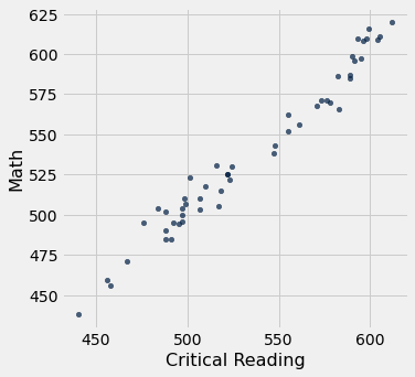
pearson_correlation(sat2014, 'Critical Reading', 'Math')
0.9847558411067432