Boostrapping
from datascience import *
%matplotlib inline
import matplotlib.pyplot as plots
plots.style.use('fivethirtyeight')
import numpy as np
import warnings
warnings.simplefilter(action='ignore', category=np.VisibleDeprecationWarning)
warnings.simplefilter(action='ignore', category=UserWarning)

from ipywidgets import interact, interactive, fixed, interact_manual
import ipywidgets as widgets
1. Median and percentiles
# A tiny set of salaries
# These are sorted, but they don't need to be to use percentile.
tiny_salaries = make_array(1317,  3909,  6015,  7467, 18632, 20828, 20950)
tiny_salaries
array([ 1317, 3909, 6015, 7467, 18632, 20828, 20950])
percentile(50, tiny_salaries)
7467
percentile(75, tiny_salaries)
20828
2. Boostrapping
# Load the 200-sample of Boston city police officers.
boston_sample = Table().read_table('data/boston-earnings-small.csv')
boston_sample.show(5)
| TITLE | REGULAR | TOTAL_GROSS |
|---|---|---|
| Police Officer | 89969 | 180643 |
| Police Officer | 83065 | 148513 |
| Police Officer | 91784 | 150195 |
| Police Officer | 25923 | 90898 |
| Police Officer | 35882 | 36068 |
... (195 rows omitted)
boston_sample.num_rows
200
boston_sample.hist('REGULAR')
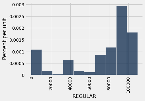
sample_median = percentile(50, boston_sample.column('REGULAR'))
sample_median
89969
def bootstrap(observed_sample, num_trials):

    bootstrap_statistics = make_array()

    for i in np.arange(0, num_trials):
        #Key: in bootstrapping we must always sample with replacement
        simulated_resample = boston_sample.sample()

        resample_statistic = percentile(50, simulated_resample.column('REGULAR')) #get the median for that one resample
        bootstrap_statistics = np.append(bootstrap_statistics, resample_statistic)

    return bootstrap_statistics
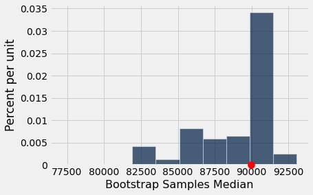
bootstrap_statistics = bootstrap(boston_sample, 10000)
# Put in Table and analyze results
results = Table().with_column('Bootstrap Samples Median', bootstrap_statistics)
results.hist()
#Plot the median of our original sample in red
plots.scatter(sample_median, 0, color='red', s=100, zorder=10, clip_on=False);
3. “Oracle” Evaluation
Oracle: pretend we are an all-knowing being and can look at the true population (which our journalist does not have access to)
We can check agaist the population for the pedagogical purposes of understanding the bootstrap. However, in the real world we would mostly likely only have the sample. And if we did have the population, we wouldn’t need to bootstrap.
population = Table().read_table('data/boston-earnings.csv')
population = population.select('TITLE', 'REGULAR', 'TOTAL_GROSS')
population = population.where('TITLE', are.equal_to('Police Officer'))
population.show(5)
| TITLE | REGULAR | TOTAL_GROSS |
|---|---|---|
| Police Officer | 0 | 1264844 |
| Police Officer | 0 | 1252991 |
| Police Officer | 100963 | 399826 |
| Police Officer | 99102 | 306588 |
| Police Officer | 91784 | 304577 |
... (1316 rows omitted)
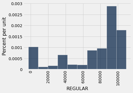
population.hist('REGULAR')
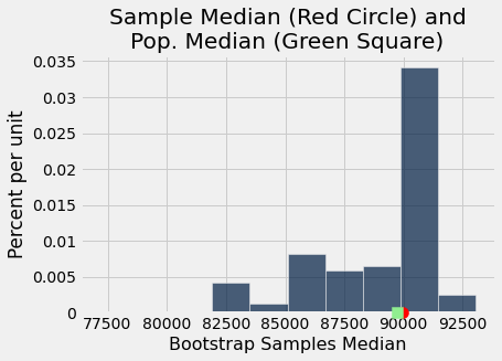
#median of the population
population_salaries = population.column('REGULAR')
true_parameter = percentile(50, population_salaries)
true_parameter
89717
# Compare the true parameter to our bootstrap estimate
results.hist()
#Plot the median of our original sample in red
plots.scatter(sample_median, 0, color='red', s=100, zorder=10, clip_on=False)
#Plot the true population parameter in green
plots.scatter(true_parameter, 0, color='lightgreen', marker='s', s=100, zorder=10, clip_on=False)
plots.title('Sample Median (Red Circle) and\nPop. Median (Green Square)');
Sensitivity to Sample Size and Number of Samples
Here’s a way to visualize how the bootstrap distribution converges to the same distribution as the one for samples from the population.
# random_seed lets us change the random numbers used to pick samples
# Basically, changing the seed let's us generated different samples.
# random_seed 0 uses boston_sample from above.  All others create new initial sample
def visualize_bootstrap(random_seed, sample_size, num_samples):
    np.random.seed(random_seed)
    if random_seed == 0:
        first_sample = boston_sample
    else:
        first_sample = population.sample(sample_size, with_replacement=False)
    medians = Table(["Type", "Median"])
    sample_medians = make_array()

    for i in np.arange(num_samples):
        sample = population.sample(sample_size)
        sample_median = percentile(50, sample.column('REGULAR'))
        medians.append([ "Realworld", sample_median ])

    for i in np.arange(num_samples):
        bootstrap_sample = first_sample.sample()
        boostrap_median = percentile(50, bootstrap_sample.column('REGULAR'))
        medians.append([ "Bootstrap", boostrap_median ])

    median_bins=np.arange(75000, 95000, 1000)
    medians.hist(group="Type", bins=median_bins)

    # Plotting parameters; you can ignore this code
    plots.scatter(true_parameter, 0.000005, color='lightgreen', marker="s", s=100, zorder=12, clip_on=False)
    plots.scatter(np.median(first_sample.column('REGULAR')), 0.000005, color='red', s=100, zorder=12, clip_on=False)
    plots.title('Bootstrap/Real World Medians\nSample Median (Red Dot); Pop Median (Green Square)\nsample size = ' + str(sample_size) + '; num samples = ' + str(num_samples));

_ = widgets.interact(visualize_bootstrap,
                     random_seed=(0,100,1),
                     sample_size=make_array(25, 50,100,200,500, 1000,2000),
                     num_samples=make_array(20,200,2000))