Causality¶

from datascience import *
%matplotlib inline
import matplotlib.pyplot as plots
plots.style.use('fivethirtyeight')
import numpy as np
import sys
import warnings
warnings.simplefilter(action='ignore', category=np.VisibleDeprecationWarning)

from ipywidgets import interact, interactive, fixed, interact_manual
import ipywidgets as widgets

1. Load maternal smoker data¶

You can read more about this data here https://www.stat.berkeley.edu/~statlabs/labs.html#babiesI

births = Table.read_table('data/baby.csv')

births

Birth Weight	Gestational Days	Maternal Age	Maternal Height	Maternal Pregnancy Weight	Maternal Smoker
120	284	27	62	100	False
113	282	33	64	135	False
128	279	28	64	115	True
108	282	23	67	125	True
136	286	25	62	93	False
138	244	33	62	178	False
132	245	23	65	140	False
120	289	25	62	125	False
143	299	30	66	136	True
140	351	27	68	120	False

... (1164 rows omitted)

births.show(4)

Birth Weight	Gestational Days	Maternal Age	Maternal Height	Maternal Pregnancy Weight	Maternal Smoker
120	284	27	62	100	False
113	282	33	64	135	False
128	279	28	64	115	True
108	282	23	67	125	True

... (1170 rows omitted)

smoking_and_birthweight = births.select('Maternal Smoker', 'Birth Weight')

smoking_and_birthweight.group('Maternal Smoker')

Maternal Smoker	count
False	715
True	459

smoking_and_birthweight.hist('Birth Weight', group='Maternal Smoker')

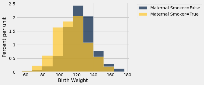
2. Test Statistic¶

means_table = smoking_and_birthweight.group('Maternal Smoker', np.mean)
means_table

Maternal Smoker	Birth Weight mean
False	123.085
True	113.819

means = means_table.column('Birth Weight mean')
observed_difference = means.item(1) - means.item(0)
observed_difference

-9.266142572024918

In keeping with the approach we laid out last lecture, we’ll focus only on absolute difference…

observed_difference = abs(means.item(1) - means.item(0))
observed_difference

9.266142572024918

def abs_difference_of_means(table, group_label, value_label):
    """
    Inputs: 
        - table: name of table
        - group_label: column label for variable you want to group 
        - value_label: column label for the variable you want to take means of 
    
    Returns: Difference of mean birth weights of the two groups
    """
    # table containing group means
    means_table = table.group(group_label, np.mean)
    
    # array of group means
    means = means_table.column(value_label + ' mean')
    
    return abs(means.item(1) - means.item(0))

Our observed difference

observed_difference = abs_difference_of_means(births, 'Maternal Smoker', "Birth Weight")
observed_difference

9.266142572024918

We can use this function on lots of columns!

abs_difference_of_means(births, 'Maternal Smoker', "Maternal Age")

0.8076725017901509

abs_difference_of_means(births, 'Maternal Smoker', "Maternal Height")

0.09058914941267915

3. Simulation Under Null Hypothesis¶

Creating Permutations of Labels¶

Just use a tiny table to show our approach…

tiny_smoking_and_birthweight = smoking_and_birthweight.take(np.arange(0,6))

shuffled_labels = tiny_smoking_and_birthweight.sample(with_replacement=False).column('Maternal Smoker')
original_and_shuffled = tiny_smoking_and_birthweight.with_column('Shuffled Label', shuffled_labels)
original_and_shuffled

Maternal Smoker	Birth Weight	Shuffled Label
False	120	False
False	113	True
True	128	False
True	108	False
False	136	False
False	138	True

A function to make a permutation!

def permutation_sample(table, group_column_name):
    """
    Returns: The table with a new "Shuffled Label" column containing
    the shuffled values of the group column.
    """
    
    # array of shuffled labels
    shuffled_labels = table.sample(with_replacement=False).column(group_column_name)
    
    # table of numerical variable and shuffled labels
    shuffled_table = table.with_column('Shuffled Label', shuffled_labels)
    
    return shuffled_table

original_and_shuffled = permutation_sample(tiny_smoking_and_birthweight, "Maternal Smoker")
original_and_shuffled

Maternal Smoker	Birth Weight	Shuffled Label
False	120	False
False	113	True
True	128	False
True	108	False
False	136	True
False	138	False

# Steve: The statistic for our reshuffled label
abs_difference_of_means(original_and_shuffled, "Shuffled Label", "Birth Weight")

1.0

And now the full table…

smoking_and_birthweight

Maternal Smoker	Birth Weight
False	120
False	113
True	128
True	108
False	136
False	138
False	132
False	120
True	143
False	140

... (1164 rows omitted)

original_and_shuffled = permutation_sample(smoking_and_birthweight, "Maternal Smoker")
original_and_shuffled

Maternal Smoker	Birth Weight	Shuffled Label
False	120	False
False	113	True
True	128	False
True	108	True
False	136	False
False	138	False
False	132	True
False	120	False
True	143	True
False	140	True

... (1164 rows omitted)

# "one trial" of our simulation 
abs_difference_of_means(original_and_shuffled, 'Shuffled Label', 'Birth Weight')

1.818306747718509

Permutation Test¶

# Steve: I removed the values column name from here -- no need to include it and do a select
# Just return the original table with a new column.
def permutation_sample(table, group_column_name):
    """
    Returns: The table with a new "Shuffled Label" column containing
    the shuffled values of the group column.
    """
    
    # array of shuffled labels
    shuffled_labels = table.sample(with_replacement=False).column(group_column_name)
    
    # table of numerical variable and shuffled labels
    shuffled_table = table.with_column('Shuffled Label', shuffled_labels)
    
    return shuffled_table

def simulate_birth_weights(num_trials):
    
    birth_weight_simulated_statistics = make_array()
    
    for i in np.arange(0, num_trials): 

        one_sample = permutation_sample(smoking_and_birthweight, "Maternal Smoker")
        statistic_one_sample = abs(abs_difference_of_means(one_sample, 
                                                           "Shuffled Label", 
                                                           "Birth Weight"))

        birth_weight_simulated_statistics = np.append(birth_weight_simulated_statistics, 
                                                      statistic_one_sample)
        
    return birth_weight_simulated_statistics

simulated_birth_weight_diffs = simulate_birth_weights(1000)

results = Table().with_column('abs(Group B Mean - Group A Mean)', simulated_birth_weight_diffs)
results.hist()
plots.scatter(observed_difference, 0, color='red', s=60, zorder=3, clip_on=False);

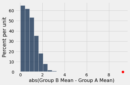
Let’s calculate the p-value (even if we can easily guess what it is here)…

sum(simulated_birth_weight_diffs >= observed_difference) / len(simulated_birth_weight_diffs)

0.0

4. Randomized Controlled Experiment¶

rct = Table.read_table('data/bta.csv')
rct.show()

Group	Result
Control	1
Control	1
Control	0
Control	0
Control	0
Control	0
Control	0
Control	0
Control	0
Control	0
Control	0
Control	0
Control	0
Control	0
Control	0
Control	0
Treatment	1
Treatment	1
Treatment	1
Treatment	1
Treatment	1
Treatment	1
Treatment	1
Treatment	1
Treatment	1
Treatment	0
Treatment	0
Treatment	0
Treatment	0
Treatment	0
Treatment	0

rct.pivot('Result', 'Group') #Recall: the default aggregation function counts the items 

Group	0.0	1.0
Control	14	2
Treatment	6	9

# This tells us the proportion in each group who improved.
rct.group('Group', np.average)

Group	Result average
Control	0.125
Treatment	0.6

Testing the Hypotheses¶

shuffled_labels = rct.sample(with_replacement=False).column('Group')
original_and_shuffled = rct.with_column('Shuffled Label', shuffled_labels)
original_and_shuffled

Group	Result	Shuffled Label
Control	1	Control
Control	1	Control
Control	0	Treatment
Control	0	Control
Control	0	Treatment
Control	0	Control
Control	0	Treatment
Control	0	Control
Control	0	Control
Control	0	Treatment

... (21 rows omitted)

# Original RCT
original_and_shuffled.select('Result', 'Group').group('Group', np.average)

Group	Result average
Control	0.125
Treatment	0.6

# Shuffled RCT from the permutation test
original_and_shuffled.select('Result', 'Shuffled Label').group('Shuffled Label', np.average)

Shuffled Label	Result average
Control	0.25
Treatment	0.466667

def difference_of_proportions(table, group_label, value_label):
    """Takes: name of table,
    column label that indicates which group the row relates to
    Returns: Difference of proportions of 1's in the two groups"""
    
    # table containing group means
    proportions_table = table.group(group_label, np.mean)
    
    # array of group means
    proportions = proportions_table.column(value_label + ' mean')
    
    return abs(proportions.item(1) - proportions.item(0))

observed_diff = difference_of_proportions(rct, 'Group', 'Result')
observed_diff

0.475

# Reuse permutation_sample, and structure same as first example.
def empirical_difference_of_proportions_distribution(num_iterations):
    simulated_diffs = make_array()

    for i in np.arange(num_iterations):
        
        one_sample = permutation_sample(rct, 'Group')
        statistic_one_sample = abs(abs_difference_of_means(one_sample, 
                                                           "Shuffled Label", 
                                                           'Result'))
        
        simulated_diffs = np.append(simulated_diffs, statistic_one_sample)
    
    return simulated_diffs

simulated_diffs = empirical_difference_of_proportions_distribution(2000)
col_name = 'Difference between Treatment and Control'
results = Table().with_column(col_name, simulated_diffs)
results.hist(left_end = observed_diff, bins=np.arange(0,0.7,0.1))
plots.scatter(observed_diff, 0, color='red', s=60, clip_on=False, zorder=3);

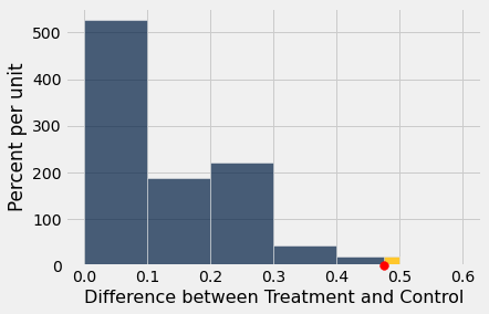
# p-value
sum(simulated_diffs >= observed_diff) / len(simulated_diffs)

0.0075

CSCI 104: Understanding Data Through Computation

Causality¶

1. Load maternal smoker data¶

2. Test Statistic¶

3. Simulation Under Null Hypothesis¶

Creating Permutations of Labels¶

Permutation Test¶

4. Randomized Controlled Experiment¶

Testing the Hypotheses¶