Hypothesis Testing
from datascience import *
%matplotlib inline
import matplotlib.pyplot as plots
plots.style.use('fivethirtyeight')
import numpy as np
import warnings
warnings.simplefilter(action='ignore', category=np.VisibleDeprecationWarning)

from ipywidgets import interact, interactive, fixed, interact_manual
import ipywidgets as widgets
1. Midterm Scores
Was Lab Section 3 graded differently than that other lab sections, or could their low average score be attributed to the random chance of the students assigned to that section?
scores = Table().read_table("data/scores_by_section.csv")
scores.group("Section")
| Section | count |
|---|---|
| 1 | 32 |
| 2 | 32 |
| 3 | 27 |
| 4 | 30 |
scores.group("Section", np.mean)
| Section | Midterm mean |
|---|---|
| 1 | 15.5938 |
| 2 | 15.125 |
| 3 | 13.1852 |
| 4 | 14.7667 |
Lab section 3’s observed average score on the midterm.
observed_scores = scores.where("Section", 3).column("Midterm")
observed_scores
array([20, 10, 20,  8, 22,  0, 15, 23, 23, 18, 15,  9, 20, 10,  0, 10, 22,
       18,  4, 16,  7, 11, 11,  0, 16, 11, 17])
observed_average = np.mean(observed_scores)
observed_average
13.185185185185185
Number of students in Lab Section 3
observed_sample_size = scores.where("Section", 3).num_rows
observed_sample_size
27
Null hypothesis model: mean of the population
Null hypothesis restated: The mean in any sample should be close to the mean in the population (the whole class)
null_hypothesis_model_parameter = np.mean(scores.column("Midterm"))
null_hypothesis_model_parameter
14.727272727272727
Difference between Lab Section 3’s average midterm score and the average midterm score across all students.
observed_midterm_statistic = abs(observed_average - null_hypothesis_model_parameter)
observed_midterm_statistic
1.5420875420875415
Abstraction: Let’s create a function that calculates a statistic as the absolute difference between the mean of a sample and the mean of a population.
def statistic_abs_diff_means(sample, population):
    """Return the absolute difference in means between a sample and a population"""
    return np.abs(np.mean(sample) - np.mean(population))
observed_midterm_statistic = statistic_abs_diff_means(observed_scores,
                                                      scores.column("Midterm"))
def sample_scores(sample_size):
    # Note: we're using with_replacement=False here because we don't
    # want to sample the same student's score twice.
    return scores.sample(sample_size, with_replacement=False).column("Midterm")
sample_scores(observed_sample_size)
array([16, 22, 20, 13,  5, 10, 10, 15, 24, 15, 13, 14, 11, 12, 11,  0, 14,
       16, 18, 25, 21, 11, 17, 24, 11, 13, 19])
def simulate_scores(observed_sample_size, num_trials):

    simulated_midterm_statistics = make_array()

    for i in np.arange(0, num_trials):

        one_sample = sample_scores(observed_sample_size)
        simulated_statistic = statistic_abs_diff_means(one_sample, scores.column("Midterm"))

        simulated_midterm_statistics = np.append(simulated_midterm_statistics,
                                                 simulated_statistic)

    return simulated_midterm_statistics
simulated_midterm_statistics = simulate_scores(observed_sample_size, 3000)
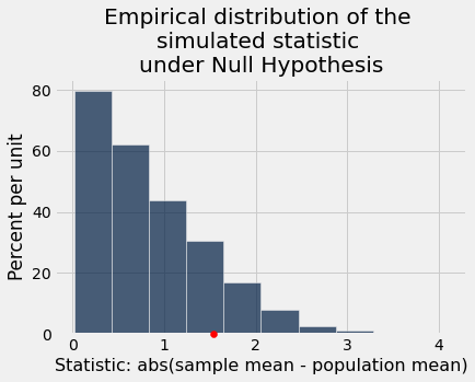
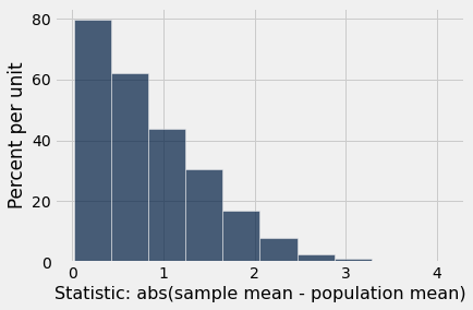
results = Table().with_columns("Statistic: abs(sample mean - population mean)",
                               simulated_midterm_statistics)
results.hist()
plots.scatter(observed_midterm_statistic, 0, color='red', zorder=10, clip_on=False);
plots.title("Empirical distribution of the \nsimulated statistic \nunder Null Hypothesis");
2. Calculating p-values
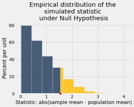
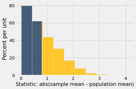
def plot_simulated_and_observed_statistics(simulated_statistics, observed_statistic):
    """
    Plots the empirical distribution of the simulated statistics, along with
    the observed data's statistic, highlighting the tail in yellow.
    """
    results = Table().with_columns("Statistic: abs(sample mean - population mean)",
                                   simulated_statistics)
    results.hist(left_end=observed_statistic)
    plots.scatter(observed_statistic, 0, color='red', zorder=10, clip_on=False);
    plots.title("Empirical distribution of the \nsimulated statistic \nunder Null Hypothesis");
plot_simulated_and_observed_statistics(simulated_midterm_statistics, observed_midterm_statistic)
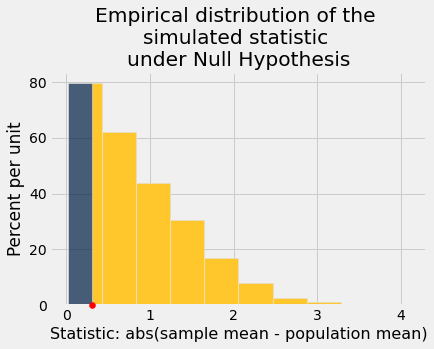
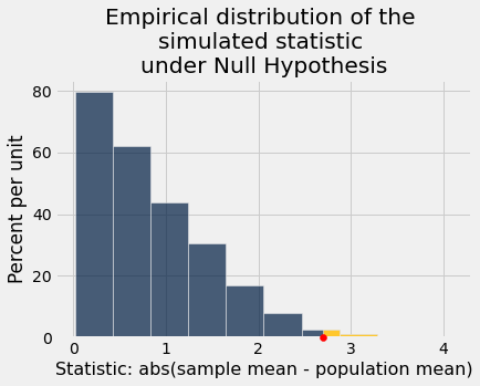
Supposed we observed other observed statistics.
plot_simulated_and_observed_statistics(simulated_midterm_statistics, 0.3)
plot_simulated_and_observed_statistics(simulated_midterm_statistics, 2.7)
Calculating p-values: Let’s compute the proportion of the histogram that is colored yellow. This captures the proportion of the simulated samples under the null hypothesis that are more unlikely than the observed data.
simulated_midterm_statistics
array([0.93939394, 0.16161616, 1.76430976, ..., 1.31986532, 0.01346801,
       1.28282828])
def calculate_pvalue(simulated_statistics, observed_statistic):
    """
    Return the proportion of the simulated statistics that are greater than
    or equal to the observed statistic
    """
    return np.count_nonzero(simulated_statistics >= observed_statistic) / len(simulated_statistics)
calculate_pvalue(simulated_midterm_statistics, observed_midterm_statistic)
0.147
Computing Percentiles
hw_scores = make_array( 31, 34, 36, 41, 43, 44, 45, 49, 51 )
percentile(50, hw_scores)
43
percentile(75, hw_scores)
45
results.hist()
percetile_55 = percentile(55, simulated_midterm_statistics)
percetile_55
0.7912457912457924
results.hist(left_end=percetile_55)
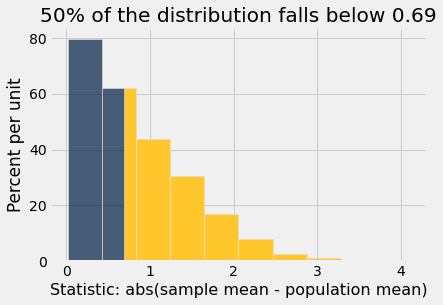
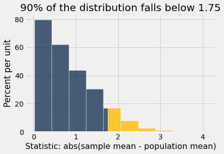
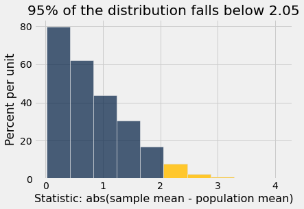
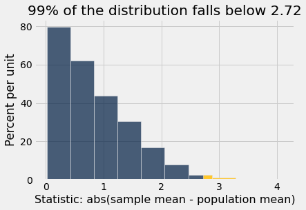
for percentile_k in make_array(50, 90, 95, 99):
    simulated_midterm_percentile = percentile(percentile_k, simulated_midterm_statistics)
    results.hist(left_end=simulated_midterm_percentile)
    plots.title(str(percentile_k)+'% of the distribution falls below '+str(np.round(simulated_midterm_percentile, 2)))
Let’s assume we are in our same set-up: our statistic is an absolute difference between the observed/simulated data and model parameters. We can then:
calculate the value of the statistic at the (conventional) 0.05 p-value and
put that statistic into our previous function
calculate_pvalue.The result in step 2 should be ~0.05!
statistic_at_five_percent_cutoff = percentile(100 - 5, simulated_midterm_statistics)
statistic_at_five_percent_cutoff
2.050505050505052
calculate_pvalue(simulated_midterm_statistics, statistic_at_five_percent_cutoff)
0.05266666666666667
Let’s write a generic function for the value of the statistic to obtain a certain p-value.
def statistic_given_pvalue(pvalue, simulated_statistics):
    """
    Return the value from the simulated statistic value for a specific p-value.
    """
    return percentile(100 - pvalue, simulated_statistics)
statistic_given_pvalue(5, simulated_midterm_statistics)
2.050505050505052
statistic_given_pvalue(1, simulated_midterm_statistics)
2.7171717171717162
3. Impact of Sample Size on p-value
def visualize_p_value_and_sample_size(sample_size, p_cutoff):

    simulated_midterm_statistics = make_array()

    for i in np.arange(0, 2000):

        one_sample = sample_scores(sample_size)
        simulated_statistic = statistic_abs_diff_means(one_sample,
                                                       scores.column("Midterm"))

        simulated_midterm_statistics = np.append(simulated_midterm_statistics,
                                             simulated_statistic)

    simulated_midterm_percentile = percentile(100 - p_cutoff,
                                              simulated_midterm_statistics)
    results = Table().with_columns("Statistic: abs(sample mean - class mean)",
                                   simulated_midterm_statistics)
    results.hist(left_end=simulated_midterm_percentile,bins=np.arange(0,6,0.2))
    plots.scatter(observed_midterm_statistic, 0, color='red', zorder=10, clip_on=False);
    plots.title(str(100 - p_cutoff)+'% of the distribution falls below '+str(np.round(simulated_midterm_percentile, 2)) + "\nSample size = "+str(sample_size))
    plots.xlim(0,5)
    plots.ylim(0,1.5)

_ = widgets.interact(visualize_p_value_and_sample_size,
                     sample_size=(10,100),
                     p_cutoff=(1,100))
Takeaway: If we have a larger sample size, the value of the test statistic to give the same p-value cut-off is less. In other words, with a larger sample size we don’t have to see as larger of extreme values to have the same statistical significance (the burden of proof that it’s not by chance is lower).