Probability and Sampling
from datascience import *
import numpy as np

%matplotlib inline
import matplotlib.pyplot as plots
plots.style.use('fivethirtyeight')

from ipywidgets import interact, interactive, fixed, interact_manual
import ipywidgets as widgets
1. Distributions
Probability Distribution
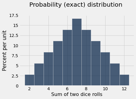
We have used probability rules to analytically write down the expected number of each possible value in order to create a probability distribution.
# Sums of all possible combinations of two dice rolls.
# (The first few entries illustrate how we constructed these combinations.)
outcomes = make_array(1+1,1+2,2+1,1+3,2+2,3+1,5,5,5,5,6,6,6,6,6,
                      7,7,7,7,7,7,8,8,8,8,8,9,9,9,9,10,10,10,11,11,12)
outcome_bins = np.arange(1.5, 13.5, 1)
Table().with_columns('Sum of two dice rolls', outcomes).hist(bins=outcome_bins)
plots.title('Probability (exact) distribution \n   ')
plots.ylim(0,0.175);
Empirical Distribution
dice = np.arange(1,7)
dice
array([1, 2, 3, 4, 5, 6])
#roll the dice twice and add the values
two_dice = np.random.choice(dice, 2)
print('two dice=', two_dice)
print('sum=', sum(two_dice))
two dice= [1 4]
sum= 5
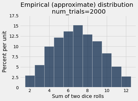
Use our standard loop idiom to build an array of the sums of two dice.
num_trials = 2000
all_outcomes = make_array()
for i in np.arange(0,num_trials):
    outcome = sum(np.random.choice(dice, 2))
    all_outcomes = np.append(all_outcomes, outcome)
simulated_results = Table().with_column('Sum of two dice rolls', all_outcomes)
simulated_results
| Sum of two dice rolls |
|---|
| 9 |
| 6 |
| 10 |
| 7 |
| 5 |
| 9 |
| 8 |
| 5 |
| 4 |
| 3 |
... (1990 rows omitted)
simulated_results.hist(bins=outcome_bins)
plots.title('Empirical (approximate) distribution \n num_trials='+str(num_trials));
plots.ylim(0,0.175);
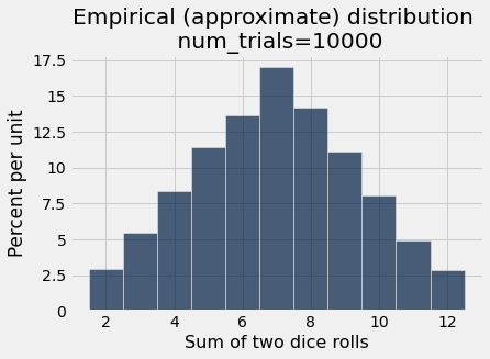
Law of Averages
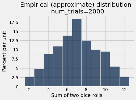
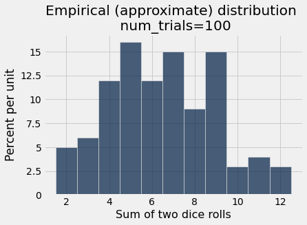
In our simulation, we have one parameter that we have the ability to control num_trials. Does this parameter matter?
To find out, we can write a function that takes as input the num_trials parameter.
def simulate_and_plot_summing_two_dice(num_trials):
    """
    Simulates rollowing two dice and repeats num_trials times, and
    Plots the empirical distribution
    """
    all_outcomes = make_array()
    for i in np.arange(0,num_trials):
        outcome = sum(np.random.choice(dice, 2))
        all_outcomes = np.append(all_outcomes, outcome)
    simulated_results = Table().with_column('Sum of two dice rolls', all_outcomes)
    simulated_results.hist(bins=outcome_bins)
    plots.title('Empirical (approximate) distribution \n num_trials='+str(num_trials));
simulate_and_plot_summing_two_dice(2000)
simulate_and_plot_summing_two_dice(100)
simulate_and_plot_summing_two_dice(500)
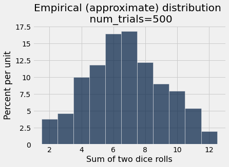
simulate_and_plot_summing_two_dice(10000)
If you run this notebook yourself, you can use the following interactive plot to see how the number of trials impacts the result.
_ = widgets.interact(simulate_and_plot_summing_two_dice, num_trials = (1,20000))
2. Random Sampling: Florida Votes in 2016
Load data for voting in Florida in 2016. These give us the true parameters if we were able to poll every person who would turn out to vote:
Proportion voting for (Trump, Clinton, Johnson, other) = (0.49, 0.478, 0.022, 0.01)
Raw counts:
Trump: 4,617,886
Clinton: 4,504,975
Johnson: 207,043
Other: 90,135
Data is based on the actual votes case in the election.
votes = Table().read_table('data/florida_2016.csv')
# the csv file uses 0,1,2,3 for the four choices, so we must convert them to candidate names
votes = votes.with_column('Vote', votes.apply(make_array("Trump", "Clinton", "Johnson", "Other").item, "Vote"))
votes.show(5)
| Vote |
|---|
| Clinton |
| Trump |
| Trump |
| Clinton |
| Trump |
... (9420034 rows omitted)
# total number of votes cast in election.
votes.num_rows
9420039
We can pick a “convenience sample”: the first 10 voters who show up in line.
votes.take(np.arange(10))
| Vote |
|---|
| Clinton |
| Trump |
| Trump |
| Clinton |
| Trump |
| Johnson |
| Clinton |
| Clinton |
| Clinton |
| Trump |
Since we actually know the votes for the full population, we can compute the true parameter.
sum(votes.column('Vote') == 'Trump') / votes.num_rows
0.49021941416590736
But suppose this is before the election and we actually can’t ask every person in the state how they will vote…
In that case, we can imagine we are a pollster, and sample 50 people.
We can use .sample(n) to randomly sample n rows from a table.
sample = votes.sample(50)
sample
| Vote |
|---|
| Clinton |
| Trump |
| Clinton |
| Trump |
| Clinton |
| Clinton |
| Trump |
| Clinton |
| Trump |
| Clinton |
... (40 rows omitted)
sum(sample.column('Vote') == 'Trump') / sample.num_rows
0.52
Sampling and computing the proportion of Trump votes in one function
def sample_proportion_vote_trump(sample_size):
    """
    Randomly samples sample_size number of rows from the votes table
    Returns the proportion that voted for Trump
    """
    sample =  votes.sample(sample_size)
    proportion_trump = sum(sample.column('Vote') == 'Trump') / sample.num_rows
    return proportion_trump
sample_proportion_vote_trump(100)
0.56
sample_proportion_vote_trump(1000)
0.471
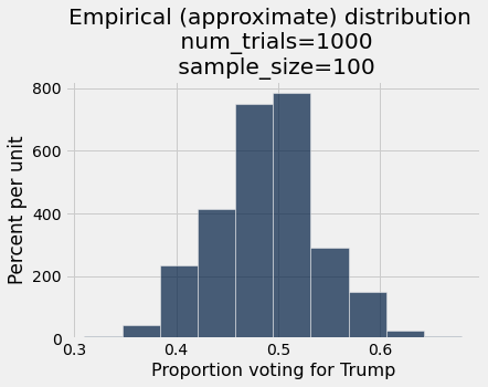
Let’s use our simulation algorithm to create an empirical distribution.
Suppose there are 1,000 polling companies and each uses a sample of 100 people.
num_trials = 1000
sample_size = 100

all_outcomes = make_array()
for i in np.arange(0,num_trials):
    outcome = sample_proportion_vote_trump(sample_size)
    all_outcomes = np.append(all_outcomes, outcome)

simulated_results = Table().with_column('Proportion voting for Trump', all_outcomes)
simulated_results.hist()

title = 'Empirical (approximate) distribution \n num_trials='+str(num_trials)+ '\n sample_size='+str(sample_size)
plots.title(title);
Let’s make a function with our two free parameters, num_trials and sample_size.
def simulate_and_plot_trump_pollster(num_trials, sample_size):
    all_outcomes = make_array()
    for i in np.arange(0,num_trials):
        outcome = sample_proportion_vote_trump(sample_size)
        all_outcomes = np.append(all_outcomes, outcome)
    simulated_results = Table().with_column('Proportion voting for Trump', all_outcomes)
    simulated_results.hist()
    title = 'Empirical (approximate) distribution \n num_trials='+str(num_trials)+ '\n sample_size='+str(sample_size)
    plots.title(title);
simulate_and_plot_trump_pollster(1000, 500)
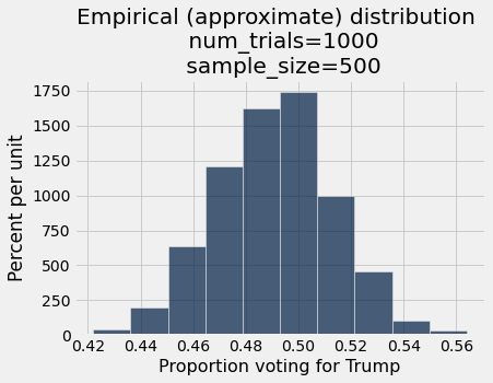
simulate_and_plot_trump_pollster(5000, 1000)
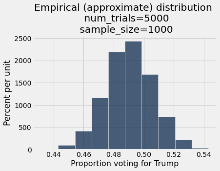
If you run this notebook yourself, you can use the following interactive plot to see how the number of trials and sample size impact the result.
_ = widgets.interact(simulate_and_plot_trump_pollster,
                     num_trials = make_array(1,10,100,1000,5000),
                     sample_size=make_array(1,10,100,1000,5000))
Big picture questions sampling:
Why wouldn’t we always just take really big of samples since they converge to the true distribution?
Big picture questions simulations:
What are we abstracting away when we’re writing code? What are we re-using over and over?