Table Examples¶

from datascience import *
%matplotlib inline
path_data = '../../../assets/data/'
import matplotlib.pyplot as plt
plt.style.use('fivethirtyeight')
import numpy as np
import warnings
warnings.simplefilter(action='ignore', category=np.VisibleDeprecationWarning)

from ipywidgets import interact, interactive, fixed, interact_manual
import ipywidgets as widgets

A pivot from our past: Temperatures in Greenland¶

We spent some time working with our Upernavik climate data.

greenland_climate = Table.read_table('data/climate_upernavik.csv').where('Year', are.above(1876))
greenland_climate = greenland_climate.relabeled('Precipitation (millimeters)', "Precip (mm)")
tidy_greenland = greenland_climate.where('Air temperature (C)', are.not_equal_to(999.99))
tidy_greenland = tidy_greenland.where('Sea level pressure (mbar)', are.not_equal_to(9999.9))
tidy_greenland

Year	Month	Air temperature (C)	Sea level pressure (mbar)	Precip (mm)
1877	1	-21.1	994.9	24
1877	2	-26.5	1008.2	26
1877	3	-17.8	1013.4	84
1877	4	-12	1023.6	6
1877	5	-1.7	1019.4	9
1877	6	1.4	1011.8	5
1877	7	4.6	1011.5	9
1877	8	5.2	1019.8	29
1877	9	3	1009	51
1877	10	-2.8	1006.2	23

... (1221 rows omitted)

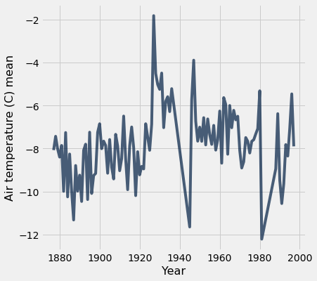
Group allows us to present average yearly temperates:

temps_by_year = tidy_greenland.group('Year', np.mean)
temps_by_year

Year	Month mean	Air temperature (C) mean	Sea level pressure (mbar) mean	Precip (mm) mean
1877	6.5	-8.075	1010.39	23.75
1878	6.5	-7.43333	1011.83	29.4167
1879	6.5	-8.01667	1010.03	7.08333
1880	6.5	-8.4	1010.75	11.5833
1881	6.5	-7.85833	1010.18	23.0833
1882	6.5	-9.99167	1011.73	8.66667
1883	6.5	-7.25833	1008.32	14.8333
1884	6.5	-10.25	1009.11	8.41667
1885	6.5	-8.25833	1011.99	10.3417
1886	6.5	-9.99167	1010.36	9

... (97 rows omitted)

We can drop the columns that aren’t meaningful or relevant, before or after the group. (Steve says he usually does it before grouping to always keep the tables as simple as possible…)

temps_by_year = temps_by_year.drop('Month mean')

temps_by_year.plot('Year', 'Air temperature (C) mean')

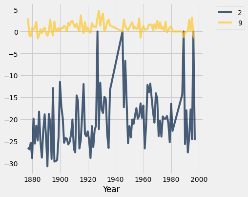
When plotting line graphs, we needed separate columns for each month. A pivot gives us a table with that format.

temps_by_month = tidy_greenland.pivot('Month', 'Year', 'Air temperature (C)', np.mean)
temps_by_month

Year	1	2	3	4	5	6	7	8	9	10	11	12
1877	-21.1	-26.5	-17.8	-12	-1.7	1.4	4.6	5.2	3	-2.8	-10	-19.2
1878	-22.9	-26.9	-19.6	-13	-5.6	1.9	3.2	4.3	-0.9	-4	-2	-3.7
1879	-13.5	-25.4	-21.3	-13	-2.7	0	5.2	5.8	-1.1	-5.5	-8.2	-16.5
1880	-22.6	-28.9	-22.7	-10.7	-3.1	2.2	5.6	2.9	0.8	-0.3	-9.4	-14.6
1881	-13.6	-19.9	-26.4	-12.8	-3.1	1.3	5.3	4.2	0.4	-2.8	-9.4	-17.5
1882	-27.6	-25.6	-24.9	-14.8	-3.2	3.1	3.3	4.1	1	-6.1	-12.1	-17.1
1883	-19.9	-21.5	-12.7	-12.8	-1.9	3	6.2	4.4	2.2	-4.1	-8.9	-21.1
1884	-26.1	-24.9	-22.7	-13.6	-6.4	1.6	5.1	3.2	-1.6	-5.1	-11.8	-20.7
1885	-15.9	-18.3	-23	-12.8	-2	-0.4	5.2	5.2	-0.8	-4.6	-13.2	-18.5
1886	-24.2	-25.2	-23.7	-18.4	-2.8	1.2	5.3	4.2	0.5	-6.3	-11.9	-18.6

... (97 rows omitted)

temps_by_month.select('Year', '2', '9').plot('Year')

Hopkins Trees¶

hopkins_trees = Table.read_table("data/hopkins-trees.csv")
hopkins_trees = hopkins_trees.drop("genus", "species")
hopkins_trees.show(10)

plot	common name	count
p00-1	Maple, striped	28
p00-1	Maple, red	8
p00-1	Maple, sugar	12
p00-1	Shadbush	17
p00-1	Birch, yellow	7
p00-1	Birch, paper	5
p00-1	Beech, American	142
p00-1	Hophornbeam	7
p00-1	Cherry, black	11
p00-1	Oak, red	6

... (3783 rows omitted)

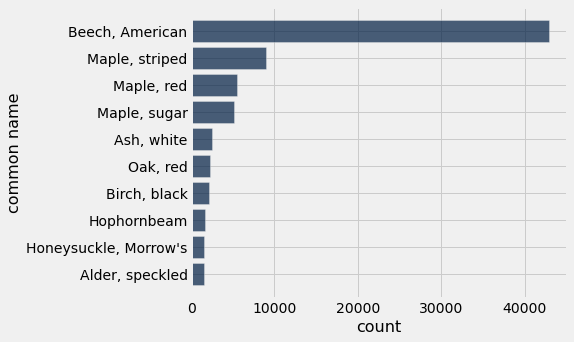
How many of each species in whole forest? Show top 10 in bar chart.¶

tree_counts = hopkins_trees.drop("plot").group("common name", sum).sort("count sum", descending=True)
tree_counts = tree_counts.relabeled('count sum', 'count')

tree_counts.take(np.arange(0,10)).barh("common name")

Create a table with counts for each type of maple for each plot.¶

maples = hopkins_trees.where('common name', are.containing('Maple'))
maples.pivot('common name', 'plot', 'count', sum)

plot	Maple, mountain	Maple, red	Maple, striped	Maple, sugar
p00-1	0	8	28	12
p00-2	0	2	43	14
p0000	0	13	0	4
p0001	3	20	11	0
p0002	0	12	1	0
p0003	0	4	41	1
p0004	0	2	9	3
p0005	0	5	17	0
p0006	0	3	26	14
p0007	0	6	123	67

... (410 rows omitted)

Create a table of red maple counts for each plot, in descending order¶

red_maples = hopkins_trees.where("common name", are.equal_to("Maple, red")).sort("count", descending=True)
red_maples

plot	common name	count
p0621	Maple, red	106
p1236	Maple, red	81
p0821	Maple, red	76
p1032	Maple, red	72
p0629	Maple, red	65
p1133	Maple, red	64
p1141	Maple, red	64
p0630	Maple, red	63
p0622	Maple, red	62
p0940	Maple, red	61

... (341 rows omitted)

Make a histogram of how many red maples are in each plot¶

red_maples.hist('count', bins=np.arange(0,100,5))

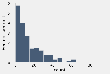
Questions:

What are the units here?
How many plots have fewer than 10 red maples?

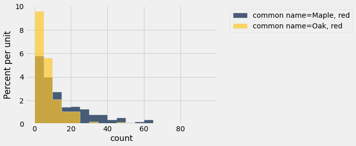
Make a histogram of both red maples and red oaks¶

reds = hopkins_trees.where("common name", are.contained_in(make_array("Maple, red", "Oak, red")))
reds.hist('count', group='common name', bins=np.arange(0,100,5))

Visualize red maples counts on a map¶

plot_info = Table.read_table("data/hopkins-plots.csv")
plot_info

plot	latitude	longitude	elevation	slope	aspect
p00-1	42.7472	-73.2759	2389	18	176
p00-2	42.7472	-73.2772	2405	22	220
p0000	42.7472	-73.2747	2343	32	139
p0001	42.7472	-73.2735	2203	80	275
p0002	42.7472	-73.2723	2022	75	136
p0003	42.7472	-73.271	1874	60	106
p0004	42.7472	-73.2698	1726	52	140
p0005	42.7472	-73.2686	1654	45	150
p0006	42.7472	-73.2673	1544	55	135
p0007	42.7472	-73.2661	1445	40	146

... (413 rows omitted)

plot_info = plot_info.select("plot", "latitude", "longitude")
plot_info

plot	latitude	longitude
p00-1	42.7472	-73.2759
p00-2	42.7472	-73.2772
p0000	42.7472	-73.2747
p0001	42.7472	-73.2735
p0002	42.7472	-73.2723
p0003	42.7472	-73.271
p0004	42.7472	-73.2698
p0005	42.7472	-73.2686
p0006	42.7472	-73.2673
p0007	42.7472	-73.2661

... (413 rows omitted)

maples_with_lat_lon = red_maples.join('plot', plot_info).select('latitude', 'longitude', 'count')
# table must be (lat, lon, colors, areas)
points = maples_with_lat_lon.with_columns("colors", "blue",
                                          "areas", 1.0 * maples_with_lat_lon.column("count"))
Circle.map_table(points).show()

Make this Notebook Trusted to load map: File -> Trust Notebook

End of lecture¶

This is as far as we got in lecture, but below are more examples you can use for practice.

Generalize to view any species using a function¶

trees_with_lat_lon = hopkins_trees.group(['plot', "common name"], sum).join("plot", plot_info)
trees_with_lat_lon = trees_with_lat_lon.relabeled('count sum', 'count')
trees_with_lat_lon

plot	common name	count	latitude	longitude
p00-1	Beech, American	142	42.7472	-73.2759
p00-1	Birch, paper	5	42.7472	-73.2759
p00-1	Birch, yellow	7	42.7472	-73.2759
p00-1	Cherry, black	11	42.7472	-73.2759
p00-1	Hophornbeam	7	42.7472	-73.2759
p00-1	Maple, red	8	42.7472	-73.2759
p00-1	Maple, striped	28	42.7472	-73.2759
p00-1	Maple, sugar	12	42.7472	-73.2759
p00-1	Oak, red	6	42.7472	-73.2759
p00-1	Shadbush	17	42.7472	-73.2759

... (3783 rows omitted)

def population_map(tree_name):
    counts = trees_with_lat_lon.where("common name", tree_name).select("latitude", "longitude", "count")
    points = counts.with_columns("colors", "blue",
                                 "areas", 1.0 * counts.column("count"))
    Circle.map_table(points).show()

population_map("Maple, red")

Make this Notebook Trusted to load map: File -> Trust Notebook

# Note: this visualization requires running the notebook on our servrer.  
# We'll see how to do that next week.
all_tree_names = trees_with_lat_lon.sort("common name", distinct=True).column("common name")
_ = widgets.interact(population_map, tree_name=all_tree_names)

Sky Scrapers¶

sky = Table.read_table('data/skyscrapers_v2.csv')
sky.show(5)

name	material	city	height	completed
One World Trade Center	mixed/composite	New York City	541.3	2014
Willis Tower	steel	Chicago	442.14	1974
432 Park Avenue	concrete	New York City	425.5	2015
Trump International Hotel & Tower	concrete	Chicago	423.22	2009
Empire State Building	steel	New York City	381	1931

... (1776 rows omitted)

Here are a bunch of questions you can try to answer about our sky scrapers data. Answers are below, but try them on your own first!

Add an age column that indicates the age of each skyscraper in years.
For each city, what’s the tallest building for each material?
For each city, what’s the height difference between the tallest steel building and the tallest concrete building?
Show a map with heights of tallest in each city.

Add an age column¶

For each city, what’s the tallest building for each material? (Try with both Group and Pivot)¶

For each city, what’s the height difference between the tallest steel building and the tallest concrete building?¶

Show a map with heights of tallest in each city¶

# Here is some lat,lon data for all cities in our skyscraper data
cities = Table().read_table('data/uscities.csv').where('population', are.above(300000))
cities = cities.select('city', 'lat', 'lng')
cities.show(5)

city	lat	lng
New York	40.6943	-73.9249
Los Angeles	34.1141	-118.407
Chicago	41.8375	-87.6866
Miami	25.784	-80.2101
Dallas	32.7935	-96.7667

... (141 rows omitted)

Sky Scrapers Answers¶

sky = Table.read_table('data/skyscrapers_v2.csv')
sky.show(5)

name	material	city	height	completed
One World Trade Center	mixed/composite	New York City	541.3	2014
Willis Tower	steel	Chicago	442.14	1974
432 Park Avenue	concrete	New York City	425.5	2015
Trump International Hotel & Tower	concrete	Chicago	423.22	2009
Empire State Building	steel	New York City	381	1931

... (1776 rows omitted)

Add an age column¶

sky = sky.with_column('age', 2022 - sky.column('completed'))
sky.show(3)

name	material	city	height	completed	age
One World Trade Center	mixed/composite	New York City	541.3	2014	8
Willis Tower	steel	Chicago	442.14	1974	48
432 Park Avenue	concrete	New York City	425.5	2015	7

... (1778 rows omitted)

For each city, what’s the tallest building for each material?¶

tallest = sky.select('material', 'city', 'height').group(make_array('city', 'material'), max)
tallest.show(5)

city	material	height max
Atlanta	concrete	264.25
Atlanta	mixed/composite	311.8
Atlanta	steel	169.47
Austin	concrete	208.15
Austin	steel	93.6

... (86 rows omitted)

sky_pivot = sky.pivot('material', 'city', 'height', max)
sky_pivot.show()

city	concrete	mixed/composite	steel
Atlanta	264.25	311.8	169.47
Austin	208.15	0	93.6
Baltimore	161.24	0	155.15
Boston	121.92	139	240.79
Charlotte	265.48	239.7	179.23
Chicago	423.22	306.94	442.14
Cincinnati	125	202.69	175
Cleveland	125	288.65	215.8
Columbus	79.25	0	169.3
Dallas	176.48	280.72	270.06
Denver	194.75	212.75	217.63
Detroit	221.49	0	173.26
Honolulu	129.8	0	130.75
Houston	217.63	305.41	302.37
Indianapolis	128.17	0	213.67
Jersey City	162.16	0	238.05
Kansas City	189.89	0	146.61
Las Vegas	350.22	195.68	164.6
Los Angeles	145.7	118.26	310.29
Miami	240.41	232.8	147.52
Miami Beach	170.39	0	0
Milwaukee	136	0	183.19
Minneapolis	203.58	241.38	144.64
New York City	425.5	541.3	381
Philadelphia	157.89	296.73	288.04
Phoenix	124.1	114	147.22
Pittsburgh	89.3	172	256.34
Portland	155.15	127.4	166.42
Sacramento	106.98	115.82	122.6
Salt Lake City	114.91	0	128.63
San Diego	151.49	144.78	152.4
San Francisco	196.6	260	237.44
Seattle	138.69	284.38	235.31
St. Louis	100.66	180.75	147.6
Sunny Isles Beach	196	0	0

For each city, what’s the height difference between the tallest steel building and the tallest concrete building?¶

sky_diff = sky_pivot.with_column(
    'difference', 
    abs(sky_pivot.column('steel') - sky_pivot.column('concrete'))
)
sky_diff

city	concrete	mixed/composite	steel	difference
Atlanta	264.25	311.8	169.47	94.78
Austin	208.15	0	93.6	114.55
Baltimore	161.24	0	155.15	6.09001
Boston	121.92	139	240.79	118.87
Charlotte	265.48	239.7	179.23	86.25
Chicago	423.22	306.94	442.14	18.92
Cincinnati	125	202.69	175	50
Cleveland	125	288.65	215.8	90.8
Columbus	79.25	0	169.3	90.05
Dallas	176.48	280.72	270.06	93.58

... (25 rows omitted)

Show a map with heights of tallest in each city¶

cities = Table().read_table('data/uscities.csv').where('population', are.above(300000))
cities = cities.select('city', 'lat', 'lng')
cities.show(5)

city	lat	lng
New York	40.6943	-73.9249
Los Angeles	34.1141	-118.407
Chicago	41.8375	-87.6866
Miami	25.784	-80.2101
Dallas	32.7935	-96.7667

... (141 rows omitted)

tallest = sky.select('material', 'city', 'height').group('city', max)
tallest = tallest.join('city', cities).select('lat', 'lng', 'city', 'height max')

points = tallest.with_columns('colors', 'blue',
                              'areas', tallest.column("height max"))
Circle.map_table(points).show()

Make this Notebook Trusted to load map: File -> Trust Notebook

CSCI 104: Understanding Data Through Computation

Table Examples¶

A pivot from our past: Temperatures in Greenland¶

Hopkins Trees¶

How many of each species in whole forest? Show top 10 in bar chart.¶

Create a table with counts for each type of maple for each plot.¶

Create a table of red maple counts for each plot, in descending order¶

Make a histogram of how many red maples are in each plot¶

Make a histogram of both red maples and red oaks¶

Visualize red maples counts on a map¶

End of lecture¶

Generalize to view any species using a function¶

Sky Scrapers¶

Add an age column¶

For each city, what’s the tallest building for each material? (Try with both Group and Pivot)¶

For each city, what’s the height difference between the tallest steel building and the tallest concrete building?¶

Show a map with heights of tallest in each city¶

Sky Scrapers Answers¶

Add an age column¶

For each city, what’s the tallest building for each material?¶

For each city, what’s the height difference between the tallest steel building and the tallest concrete building?¶

Show a map with heights of tallest in each city¶