Pivots and Joins
from datascience import *
import numpy as np

%matplotlib inline
import matplotlib.pyplot as plots
plots.style.use('fivethirtyeight')
import warnings
warnings.simplefilter(action='ignore',category=np.VisibleDeprecationWarning)
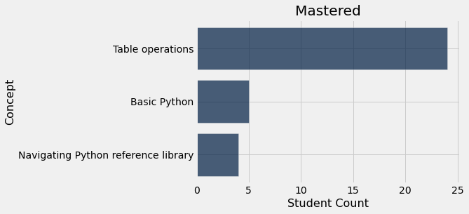
Responses from student survey
# We retained an answer if 2+ students gave that answer
mastered_concepts = Table().with_columns(
'Concept', make_array('Table operations', 'Basic Python', 'Navigating Python reference library'),
'Student Count', make_array(24, 5, 4)
)
mastered_concepts.sort('Student Count', descending=True).barh('Concept', 'Student Count')
plots.title('Mastered');
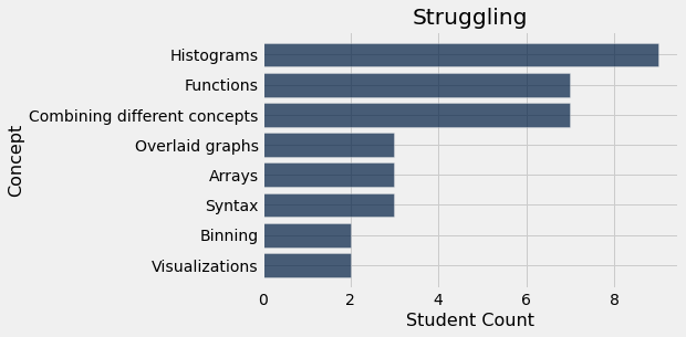
# We retained an answer if 2+ students gave that answer
struggling_concepts = Table().with_columns(
'Concept', make_array('Functions', 'Histograms', 'Binning', 'Overlaid graphs', 'Combining different concepts', 'Arrays', 'Syntax', 'Visualizations'),
'Student Count', make_array(7, 9, 2, 3, 7, 3, 3, 2)
)
struggling_concepts.sort('Student Count', descending=True).barh('Concept', 'Student Count')
plots.title('Struggling');
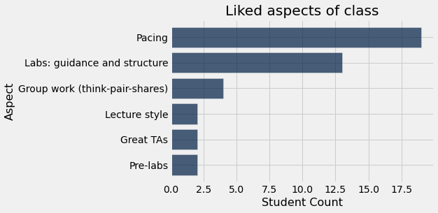
# We retained an answer if 2+ students gave that answer
liked_aspects = Table().with_columns(
'Aspect', make_array('Labs: guidance and structure', 'Pacing', 'Lecture style', 'Group work (think-pair-shares)', 'Great TAs', 'Pre-labs'),
'Student Count', make_array(13, 19, 2, 4, 2, 2)
)
liked_aspects.sort('Student Count', descending=True).barh('Aspect', 'Student Count')
plots.title('Liked aspects of class');
Review groups

“President Barack Obama receives a gift from Saudi King Abdullah at the start of their bilateral meeting in Riyadh, Saudi Arabia, on June 3, 2009. The large gold medallion was among several gifts given that day that were valued at $34,500, the State Department later said” –CBS News
# Read in all gifts, and tidy up table by removing nan values and relabeling columns
all_gifts = Table().read_table('data/obama-gifts.csv')
all_gifts = all_gifts.where('donor_country', are.not_equal_to('nan')) #clean up and remove the nans
all_gifts = all_gifts.select('year_received', 'donor_country', 'value_usd')
all_gifts = all_gifts.relabeled('year_received', 'Year')
all_gifts = all_gifts.relabeled('donor_country', 'Country')
all_gifts = all_gifts.relabeled('value_usd', 'Value')
all_gifts
| Year | Country | Value |
|---|---|---|
| 2009 | Mexico | 400 |
| 2009 | Japan | 1495 |
| 2009 | United Kingdom | 16510 |
| 2009 | Algeria | 500 |
| 2009 | Denmark | 388 |
| 2009 | Russia | 415 |
| 2009 | Germany | 760 |
| 2009 | Czechia | 1460 |
| 2009 | Turkey | 1550 |
| 2009 | Iraq | 1850 |
... (603 rows omitted)
# We'll also create a small subset of our Obama Gifts dataset.
# It contains 3 countries, 3 years, 7 gifts
gifts = all_gifts.where('Year', are.contained_in([2009,2010,2011,2012]))
gifts = gifts.where('Country', are.contained_in(make_array('Denmark', 'Egypt', 'Finland')))
gifts = gifts.sort('Year')
gifts
| Year | Country | Value |
|---|---|---|
| 2009 | Denmark | 388 |
| 2009 | Egypt | 630 |
| 2009 | Denmark | 340 |
| 2010 | Finland | 445 |
| 2010 | Egypt | 356 |
| 2010 | Egypt | 380 |
| 2011 | Denmark | 485 |
gifts.group('Year')
| Year | count |
|---|---|
| 2009 | 3 |
| 2010 | 3 |
| 2011 | 1 |
gifts.group('Country')
| Country | count |
|---|---|
| Denmark | 3 |
| Egypt | 3 |
| Finland | 1 |
gifts.group('Year', sum)
| Year | Country sum | Value sum |
|---|---|---|
| 2009 | 1358 | |
| 2010 | 1181 | |
| 2011 | 485 |
all_gifts.group('Year', sum)
| Year | Country sum | Value sum |
|---|---|---|
| 2009 | 571164 | |
| 2010 | 122626 | |
| 2011 | 233730 | |
| 2012 | 75307.8 | |
| 2013 | 198508 | |
| 2014 | 1.40138e+06 | |
| 2015 | 1.10529e+06 | |
| 2016 | 147903 |
gifts.group('Country', max)
| Country | Year max | Value max |
|---|---|---|
| Denmark | 2011 | 485 |
| Egypt | 2010 | 630 |
| Finland | 2010 | 445 |
gifts.group(make_array('Year', 'Country'), sum)
| Year | Country | Value sum |
|---|---|---|
| 2009 | Denmark | 728 |
| 2009 | Egypt | 630 |
| 2010 | Egypt | 736 |
| 2010 | Finland | 445 |
| 2011 | Denmark | 485 |
gifts.group(make_array('Year', 'Country'))
| Year | Country | count |
|---|---|---|
| 2009 | Denmark | 2 |
| 2009 | Egypt | 1 |
| 2010 | Egypt | 2 |
| 2010 | Finland | 1 |
| 2011 | Denmark | 1 |
Pivots
Summarize data that has been grouped by two variables in a grid.
gifts
| Year | Country | Value |
|---|---|---|
| 2009 | Denmark | 388 |
| 2009 | Egypt | 630 |
| 2009 | Denmark | 340 |
| 2010 | Finland | 445 |
| 2010 | Egypt | 356 |
| 2010 | Egypt | 380 |
| 2011 | Denmark | 485 |
gifts.pivot('Year', 'Country')
| Country | 2009 | 2010 | 2011 |
|---|---|---|---|
| Denmark | 2 | 0 | 1 |
| Egypt | 1 | 2 | 0 |
| Finland | 0 | 1 | 0 |
gifts.pivot('Country', 'Year')
| Year | Denmark | Egypt | Finland |
|---|---|---|---|
| 2009 | 2 | 1 | 0 |
| 2010 | 0 | 2 | 1 |
| 2011 | 1 | 0 | 0 |
gifts.pivot('Year', 'Country', 'Value', sum)
| Country | 2009 | 2010 | 2011 |
|---|---|---|---|
| Denmark | 728 | 0 | 485 |
| Egypt | 630 | 736 | 0 |
| Finland | 0 | 445 | 0 |
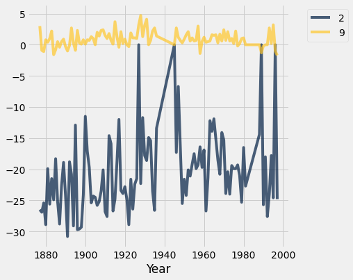
A pivot from our past: Temperatures in Greenland
We spent some time working with our Upernavik climate data.
greenland_climate = Table.read_table('data/climate_upernavik.csv').where('Year', are.above(1876))
greenland_climate = greenland_climate.relabeled('Precipitation (millimeters)', "Precip (mm)")
tidy_greenland = greenland_climate.where('Air temperature (C)', are.not_equal_to(999.99))
tidy_greenland = tidy_greenland.where('Sea level pressure (mbar)', are.not_equal_to(9999.9))
tidy_greenland
| Year | Month | Air temperature (C) | Sea level pressure (mbar) | Precip (mm) |
|---|---|---|---|---|
| 1877 | 1 | -21.1 | 994.9 | 24 |
| 1877 | 2 | -26.5 | 1008.2 | 26 |
| 1877 | 3 | -17.8 | 1013.4 | 84 |
| 1877 | 4 | -12 | 1023.6 | 6 |
| 1877 | 5 | -1.7 | 1019.4 | 9 |
| 1877 | 6 | 1.4 | 1011.8 | 5 |
| 1877 | 7 | 4.6 | 1011.5 | 9 |
| 1877 | 8 | 5.2 | 1019.8 | 29 |
| 1877 | 9 | 3 | 1009 | 51 |
| 1877 | 10 | -2.8 | 1006.2 | 23 |
... (1221 rows omitted)
When plotting line graphs, we needed separate columns for each month. A pivot gives us a table with that format.
temps_by_month = tidy_greenland.pivot('Month', 'Year', 'Air temperature (C)', np.mean)
temps_by_month
| Year | 1 | 2 | 3 | 4 | 5 | 6 | 7 | 8 | 9 | 10 | 11 | 12 |
|---|---|---|---|---|---|---|---|---|---|---|---|---|
| 1877 | -21.1 | -26.5 | -17.8 | -12 | -1.7 | 1.4 | 4.6 | 5.2 | 3 | -2.8 | -10 | -19.2 |
| 1878 | -22.9 | -26.9 | -19.6 | -13 | -5.6 | 1.9 | 3.2 | 4.3 | -0.9 | -4 | -2 | -3.7 |
| 1879 | -13.5 | -25.4 | -21.3 | -13 | -2.7 | 0 | 5.2 | 5.8 | -1.1 | -5.5 | -8.2 | -16.5 |
| 1880 | -22.6 | -28.9 | -22.7 | -10.7 | -3.1 | 2.2 | 5.6 | 2.9 | 0.8 | -0.3 | -9.4 | -14.6 |
| 1881 | -13.6 | -19.9 | -26.4 | -12.8 | -3.1 | 1.3 | 5.3 | 4.2 | 0.4 | -2.8 | -9.4 | -17.5 |
| 1882 | -27.6 | -25.6 | -24.9 | -14.8 | -3.2 | 3.1 | 3.3 | 4.1 | 1 | -6.1 | -12.1 | -17.1 |
| 1883 | -19.9 | -21.5 | -12.7 | -12.8 | -1.9 | 3 | 6.2 | 4.4 | 2.2 | -4.1 | -8.9 | -21.1 |
| 1884 | -26.1 | -24.9 | -22.7 | -13.6 | -6.4 | 1.6 | 5.1 | 3.2 | -1.6 | -5.1 | -11.8 | -20.7 |
| 1885 | -15.9 | -18.3 | -23 | -12.8 | -2 | -0.4 | 5.2 | 5.2 | -0.8 | -4.6 | -13.2 | -18.5 |
| 1886 | -24.2 | -25.2 | -23.7 | -18.4 | -2.8 | 1.2 | 5.3 | 4.2 | 0.5 | -6.3 | -11.9 | -18.6 |
... (97 rows omitted)
temps_by_month.select('Year', '2', '9').plot('Year')
Group vs. Pivot
When is it an advantage to use pivot over group and vice versa?
Joins
Let’s hand pick a few of our favorite gifts.
best_gifts = gifts.take(0,1,2,3).drop("Year")
best_gifts
| Country | Value |
|---|---|
| Denmark | 388 |
| Egypt | 630 |
| Denmark | 340 |
| Finland | 445 |
If you’re curious what they are, here are shortened descriptions for the four we chose.
best_gifts.with_columns("Gift description",
                        make_array('Book "Restoring the Military Balance"',
                                   'Yellow alabaster bowl',
                                   'Photograph of Her Majesty and His Royal Highness',
                                   'Hand-blown blue glass bird'))
| Country | Value | Gift description |
|---|---|---|
| Denmark | 388 | Book "Restoring the Military Balance" |
| Egypt | 630 | Yellow alabaster bowl |
| Denmark | 340 | Photograph of Her Majesty and His Royal Highness |
| Finland | 445 | Hand-blown blue glass bird |
Here is some other info about countries, specifically the GDP from each country during Obama’s first year in office. (GDP is gross domestic product, a measure of the value of the final goods and services produced in a country.)
# Values taken from World Bank and IMF sites.
# https://data.worldbank.org/indicator/NY.GDP.MKTP.CD
# https://www.imf.org/en/Publications/WEO/weo-database/2022/April/download-entire-database
gdp = Table().with_columns(
    'Country Name', make_array('Denmark', 'Egypt', 'Egypt', 'Greece'),
    'GDP (Billion $)', make_array(321, 189, 198, 331),
    'Source', make_array('World Bank', 'World Bank', 'IMF', 'World Bank'))
gdp
| Country Name | GDP (Billion $) | Source |
|---|---|---|
| Denmark | 321 | World Bank |
| Egypt | 189 | World Bank |
| Egypt | 198 | IMF |
| Greece | 331 | World Bank |
Can we combine best_gifts with info about the countries like GDP?
Join will let us merge data from two tables by pairing together rows from each that share a common property. Here we’ll merge a table of gifts with a table of GDP information about the countres giving gifts.
# Values taken from World Bank and IMF sites.
# https://data.worldbank.org/indicator/NY.GDP.MKTP.CD
# https://www.imf.org/en/Publications/WEO/weo-database/2022/April/download-entire-database
gdp = Table().with_columns(
    'Country Name', make_array('Denmark', 'Egypt', 'Egypt', 'Greece'),
    'GDP (Billion $)', make_array(321, 189, 198, 331),
    'Source', make_array('World Bank', 'World Bank', 'IMF', 'World Bank'))
gdp
| Country Name | GDP (Billion $) | Source |
|---|---|---|
| Denmark | 321 | World Bank |
| Egypt | 189 | World Bank |
| Egypt | 198 | IMF |
| Greece | 331 | World Bank |
best_gifts.join('Country', gdp, 'Country Name')
| Country | Value | GDP (Billion $) | Source |
|---|---|---|---|
| Denmark | 388 | 321 | World Bank |
| Denmark | 340 | 321 | World Bank |
| Egypt | 630 | 189 | World Bank |
| Egypt | 630 | 198 | IMF |
Open-ended exploration
Suppose we had the following question: Is there any relationship between a country’s GDP and the sum total of the amount of gifts they gave to President Obama?
The World Bank provides GDP data we can use.
gdp = Table().read_table('data/gdp.csv')
gdp.take(np.arange(10,20))
| Country Name | Country Code | Indicator Name | Indicator Code | 1960 | 1961 | 1962 | 1963 | 1964 | 1965 | 1966 | 1967 | 1968 | 1969 | 1970 | 1971 | 1972 | 1973 | 1974 | 1975 | 1976 | 1977 | 1978 | 1979 | 1980 | 1981 | 1982 | 1983 | 1984 | 1985 | 1986 | 1987 | 1988 | 1989 | 1990 | 1991 | 1992 | 1993 | 1994 | 1995 | 1996 | 1997 | 1998 | 1999 | 2000 | 2001 | 2002 | 2003 | 2004 | 2005 | 2006 | 2007 | 2008 | 2009 | 2010 | 2011 | 2012 | 2013 | 2014 | 2015 | 2016 | 2017 | 2018 | 2019 | 2020 | 2021 | Unnamed: 66 |
|---|---|---|---|---|---|---|---|---|---|---|---|---|---|---|---|---|---|---|---|---|---|---|---|---|---|---|---|---|---|---|---|---|---|---|---|---|---|---|---|---|---|---|---|---|---|---|---|---|---|---|---|---|---|---|---|---|---|---|---|---|---|---|---|---|---|---|
| Armenia | ARM | GDP (current US$) | NY.GDP.MKTP.CD | nan | nan | nan | nan | nan | nan | nan | nan | nan | nan | nan | nan | nan | nan | nan | nan | nan | nan | nan | nan | nan | nan | nan | nan | nan | nan | nan | nan | nan | nan | 2.25684e+09 | 2.06987e+09 | 1.27284e+09 | 1.20131e+09 | 1.31516e+09 | 1.46832e+09 | 1.59697e+09 | 1.63949e+09 | 1.89373e+09 | 1.84548e+09 | 1.91156e+09 | 2.11847e+09 | 2.37634e+09 | 2.80706e+09 | 3.57662e+09 | 4.90047e+09 | 6.38445e+09 | 9.2063e+09 | 1.1662e+10 | 8.64794e+09 | 9.26028e+09 | 1.01421e+10 | 1.06193e+10 | 1.11215e+10 | 1.16095e+10 | 1.05533e+10 | 1.05461e+10 | 1.15275e+10 | 1.24579e+10 | 1.36193e+10 | 1.26412e+10 | 1.38612e+10 | nan |
| American Samoa | ASM | GDP (current US$) | NY.GDP.MKTP.CD | nan | nan | nan | nan | nan | nan | nan | nan | nan | nan | nan | nan | nan | nan | nan | nan | nan | nan | nan | nan | nan | nan | nan | nan | nan | nan | nan | nan | nan | nan | nan | nan | nan | nan | nan | nan | nan | nan | nan | nan | nan | nan | 5.12e+08 | 5.24e+08 | 5.09e+08 | 5e+08 | 4.93e+08 | 5.18e+08 | 5.6e+08 | 6.75e+08 | 5.73e+08 | 5.7e+08 | 6.4e+08 | 6.38e+08 | 6.43e+08 | 6.73e+08 | 6.71e+08 | 6.12e+08 | 6.39e+08 | 6.48e+08 | 7.09e+08 | nan | nan |
| Antigua and Barbuda | ATG | GDP (current US$) | NY.GDP.MKTP.CD | nan | nan | nan | nan | nan | nan | nan | nan | nan | nan | nan | nan | nan | nan | nan | nan | nan | 7.74968e+07 | 8.78793e+07 | 1.0908e+08 | 1.31431e+08 | 1.47842e+08 | 1.64369e+08 | 1.82144e+08 | 2.08373e+08 | 2.40924e+08 | 2.9044e+08 | 3.37175e+08 | 3.98638e+08 | 4.38795e+08 | 4.5947e+08 | 4.81707e+08 | 4.99281e+08 | 5.35174e+08 | 5.8943e+08 | 5.77281e+08 | 6.3373e+08 | 6.80619e+08 | 7.27859e+08 | 7.662e+08 | 8.2637e+08 | 8.00481e+08 | 8.14381e+08 | 8.56396e+08 | 9.1973e+08 | 1.02296e+09 | 1.15766e+09 | 1.31276e+09 | 1.37007e+09 | 1.22833e+09 | 1.1487e+09 | 1.13764e+09 | 1.19995e+09 | 1.18145e+09 | 1.24973e+09 | 1.33669e+09 | 1.43659e+09 | 1.46798e+09 | 1.60594e+09 | 1.68753e+09 | 1.37028e+09 | 1.47113e+09 | nan |
| Australia | AUS | GDP (current US$) | NY.GDP.MKTP.CD | 1.86068e+10 | 1.96831e+10 | 1.99227e+10 | 2.15399e+10 | 2.38011e+10 | 2.59772e+10 | 2.73099e+10 | 3.04446e+10 | 3.2717e+10 | 3.66861e+10 | 4.13372e+10 | 4.52223e+10 | 5.20514e+10 | 6.3845e+10 | 8.89816e+10 | 9.73331e+10 | 1.05101e+11 | 1.10388e+11 | 1.18536e+11 | 1.34941e+11 | 1.50032e+11 | 1.76953e+11 | 1.94105e+11 | 1.77334e+11 | 1.93594e+11 | 1.80574e+11 | 1.82368e+11 | 1.894e+11 | 2.36066e+11 | 2.99768e+11 | 3.11327e+11 | 3.25903e+11 | 3.2548e+11 | 3.12126e+11 | 3.22807e+11 | 3.67916e+11 | 4.0109e+11 | 4.35324e+11 | 3.99404e+11 | 3.89099e+11 | 4.15576e+11 | 3.79084e+11 | 3.95343e+11 | 4.67391e+11 | 6.14166e+11 | 6.95075e+11 | 7.47556e+11 | 8.53955e+11 | 1.05513e+12 | 9.28043e+11 | 1.14759e+12 | 1.39791e+12 | 1.54651e+12 | 1.57634e+12 | 1.4675e+12 | 1.35053e+12 | 1.20669e+12 | 1.32688e+12 | 1.42853e+12 | 1.39195e+12 | 1.32784e+12 | 1.54266e+12 | nan |
| Austria | AUT | GDP (current US$) | NY.GDP.MKTP.CD | 6.59269e+09 | 7.31175e+09 | 7.75611e+09 | 8.37418e+09 | 9.16998e+09 | 9.99407e+09 | 1.08877e+10 | 1.15794e+10 | 1.24406e+10 | 1.35828e+10 | 1.5373e+10 | 1.78585e+10 | 2.20596e+10 | 2.95155e+10 | 3.51893e+10 | 4.00592e+10 | 4.296e+10 | 5.15458e+10 | 6.20523e+10 | 7.39373e+10 | 8.20589e+10 | 7.10342e+10 | 7.12753e+10 | 7.2121e+10 | 6.79853e+10 | 6.93868e+10 | 9.90362e+10 | 1.24168e+11 | 1.33339e+11 | 1.33106e+11 | 1.66463e+11 | 1.73794e+11 | 1.95078e+11 | 1.9038e+11 | 2.03535e+11 | 2.41038e+11 | 2.37251e+11 | 2.1279e+11 | 2.1826e+11 | 2.17259e+11 | 1.9729e+11 | 1.97509e+11 | 2.14395e+11 | 2.62274e+11 | 3.01458e+11 | 3.16092e+11 | 3.3628e+11 | 3.89186e+11 | 4.32052e+11 | 4.01759e+11 | 3.92275e+11 | 4.31685e+11 | 4.09402e+11 | 4.30191e+11 | 4.42585e+11 | 3.81971e+11 | 3.95837e+11 | 4.17261e+11 | 4.55168e+11 | 4.45012e+11 | 4.33258e+11 | 4.77082e+11 | nan |
| Azerbaijan | AZE | GDP (current US$) | NY.GDP.MKTP.CD | nan | nan | nan | nan | nan | nan | nan | nan | nan | nan | nan | nan | nan | nan | nan | nan | nan | nan | nan | nan | nan | nan | nan | nan | nan | nan | nan | nan | nan | nan | 8.85801e+09 | 8.79237e+09 | 4.46306e+08 | 1.57e+09 | 1.19331e+09 | 2.41736e+09 | 3.17633e+09 | 3.96224e+09 | 4.44637e+09 | 4.58143e+09 | 5.2728e+09 | 5.70772e+09 | 6.23586e+09 | 7.27675e+09 | 8.68037e+09 | 1.32457e+10 | 2.0983e+10 | 3.30503e+10 | 4.88525e+10 | 4.42915e+10 | 5.29093e+10 | 6.59516e+10 | 6.96839e+10 | 7.41644e+10 | 7.52443e+10 | 5.30744e+10 | 3.78675e+10 | 4.08656e+10 | 4.71129e+10 | 4.81742e+10 | 4.2693e+10 | 5.46222e+10 | nan |
| Burundi | BDI | GDP (current US$) | NY.GDP.MKTP.CD | 1.96e+08 | 2.03e+08 | 2.135e+08 | 2.3275e+08 | 2.6075e+08 | 1.58995e+08 | 1.65445e+08 | 1.78297e+08 | 1.832e+08 | 1.90206e+08 | 2.42733e+08 | 2.52842e+08 | 2.46805e+08 | 3.0434e+08 | 3.45263e+08 | 4.20987e+08 | 4.48413e+08 | 5.47536e+08 | 6.10226e+08 | 7.82497e+08 | 9.19727e+08 | 9.69047e+08 | 1.01322e+09 | 1.08293e+09 | 9.87144e+08 | 1.14998e+09 | 1.20173e+09 | 1.13147e+09 | 1.0824e+09 | 1.11392e+09 | 1.1321e+09 | 1.1674e+09 | 1.08304e+09 | 9.38633e+08 | 9.25031e+08 | 1.00043e+09 | 8.69034e+08 | 9.72896e+08 | 8.93771e+08 | 8.08077e+08 | 8.70486e+08 | 8.76795e+08 | 8.25394e+08 | 7.84654e+08 | 9.15257e+08 | 1.11711e+09 | 1.27338e+09 | 1.3562e+09 | 1.61184e+09 | 1.78146e+09 | 2.03214e+09 | 2.23582e+09 | 2.33334e+09 | 2.45161e+09 | 2.70578e+09 | 3.104e+09 | 2.63932e+09 | 2.71232e+09 | 2.66012e+09 | 2.58127e+09 | 2.78051e+09 | 2.90203e+09 | nan |
| Belgium | BEL | GDP (current US$) | NY.GDP.MKTP.CD | 1.16587e+10 | 1.24001e+10 | 1.3264e+10 | 1.426e+10 | 1.59601e+10 | 1.73715e+10 | 1.86519e+10 | 1.9992e+10 | 2.13764e+10 | 2.37107e+10 | 2.67062e+10 | 2.98217e+10 | 3.72094e+10 | 4.77438e+10 | 5.60331e+10 | 6.56782e+10 | 7.11139e+10 | 8.28399e+10 | 1.01247e+11 | 1.16315e+11 | 1.26829e+11 | 1.0473e+11 | 9.20959e+10 | 8.71842e+10 | 8.33495e+10 | 8.62683e+10 | 1.20019e+11 | 1.49394e+11 | 1.62299e+11 | 1.64221e+11 | 2.05332e+11 | 2.10511e+11 | 2.34782e+11 | 2.24722e+11 | 2.44884e+11 | 2.88026e+11 | 2.79201e+11 | 2.52708e+11 | 2.58528e+11 | 2.58246e+11 | 2.36792e+11 | 2.36746e+11 | 2.58384e+11 | 3.18083e+11 | 3.69215e+11 | 3.85715e+11 | 4.0826e+11 | 4.70922e+11 | 5.17328e+11 | 4.83254e+11 | 4.81421e+11 | 5.2333e+11 | 4.96153e+11 | 5.21791e+11 | 5.3539e+11 | 4.62336e+11 | 4.76063e+11 | 5.02765e+11 | 5.43347e+11 | 5.35376e+11 | 5.21677e+11 | 5.99879e+11 | nan |
| Benin | BEN | GDP (current US$) | NY.GDP.MKTP.CD | 2.26196e+08 | 2.35668e+08 | 2.36435e+08 | 2.53928e+08 | 2.69819e+08 | 2.89909e+08 | 3.02925e+08 | 3.06222e+08 | 3.26323e+08 | 3.30748e+08 | 3.33628e+08 | 3.35073e+08 | 4.10332e+08 | 5.04376e+08 | 5.54655e+08 | 6.7687e+08 | 6.98408e+08 | 7.5005e+08 | 9.28843e+08 | 1.18623e+09 | 1.40525e+09 | 1.29112e+09 | 1.26778e+09 | 1.09535e+09 | 1.05113e+09 | 1.04571e+09 | 1.3361e+09 | 1.56241e+09 | 1.62025e+09 | 1.50229e+09 | 1.95997e+09 | 1.98644e+09 | 1.69532e+09 | 2.27456e+09 | 1.59808e+09 | 2.16963e+09 | 2.36112e+09 | 2.2683e+09 | 2.45509e+09 | 3.67739e+09 | 3.51999e+09 | 3.66622e+09 | 4.19434e+09 | 5.34926e+09 | 6.19027e+09 | 6.56765e+09 | 7.03411e+09 | 8.16905e+09 | 9.78774e+09 | 9.73863e+09 | 9.53534e+09 | 1.06933e+10 | 1.11414e+10 | 1.25178e+10 | 1.32845e+10 | 1.13882e+10 | 1.18211e+10 | 1.27017e+10 | 1.42624e+10 | 1.43917e+10 | 1.56515e+10 | 1.77856e+10 | nan |
| Burkina Faso | BFA | GDP (current US$) | NY.GDP.MKTP.CD | 3.30443e+08 | 3.50247e+08 | 3.79567e+08 | 3.94041e+08 | 4.10322e+08 | 4.22917e+08 | 4.3389e+08 | 4.50754e+08 | 4.60443e+08 | 4.78299e+08 | 4.58404e+08 | 4.82411e+08 | 5.78596e+08 | 6.74774e+08 | 7.51133e+08 | 9.39973e+08 | 9.76547e+08 | 1.13122e+09 | 1.47558e+09 | 1.74848e+09 | 1.92872e+09 | 1.77584e+09 | 1.75445e+09 | 1.60028e+09 | 1.45988e+09 | 1.55249e+09 | 2.0363e+09 | 2.36983e+09 | 2.61604e+09 | 2.61559e+09 | 3.1013e+09 | 3.13505e+09 | 3.35669e+09 | 3.19954e+09 | 1.89529e+09 | 2.37952e+09 | 2.58655e+09 | 2.44767e+09 | 2.8049e+09 | 3.38957e+09 | 2.96837e+09 | 3.19037e+09 | 3.62235e+09 | 4.74077e+09 | 5.45169e+09 | 6.14635e+09 | 6.54742e+09 | 7.62572e+09 | 9.45144e+09 | 9.4507e+09 | 1.01096e+10 | 1.20803e+10 | 1.2561e+10 | 1.34443e+10 | 1.3943e+10 | 1.18322e+10 | 1.28334e+10 | 1.4107e+10 | 1.58901e+10 | 1.61782e+10 | 1.79336e+10 | 1.97376e+10 | nan |
gdp_2008 = Table().with_columns(
    'Country Name', gdp.column('Country Name'),
    '2008 GDP Billion USD', gdp.column('2008') / 1e9
)
gdp_2008.take(np.arange(10,20))
| Country Name | 2008 GDP Billion USD |
|---|---|
| Armenia | 11.662 |
| American Samoa | 0.56 |
| Antigua and Barbuda | 1.37007 |
| Australia | 1055.13 |
| Austria | 432.052 |
| Azerbaijan | 48.8525 |
| Burundi | 1.61184 |
| Belgium | 517.328 |
| Benin | 9.78774 |
| Burkina Faso | 9.45144 |
gifts_by_country = all_gifts.drop('Year').group('Country', sum)
gifts_by_country
| Country | Value sum |
|---|---|
| Afghanistan | 9263 |
| Algeria | 4312.28 |
| Argentina | 3977.98 |
| Armenia | 2985 |
| Australia | 4365.48 |
| Austria | 1275 |
| Azerbaijan | 11503 |
| Bahrain | 10494 |
| Bangladesh | 390 |
| Bavaria | 1928.71 |
... (113 rows omitted)
joined = gifts_by_country.join('Country', gdp_2008, 'Country Name')
joined
| Country | Value sum | 2008 GDP Billion USD |
|---|---|---|
| Afghanistan | 9263 | 10.1093 |
| Algeria | 4312.28 | 171.001 |
| Argentina | 3977.98 | 361.558 |
| Armenia | 2985 | 11.662 |
| Australia | 4365.48 | 1055.13 |
| Austria | 1275 | 432.052 |
| Azerbaijan | 11503 | 48.8525 |
| Bahrain | 10494 | 25.7109 |
| Bangladesh | 390 | 91.6313 |
| Benin | 12289.9 | 9.78774 |
... (91 rows omitted)
joined.scatter('2008 GDP Billion USD', 'Value sum')
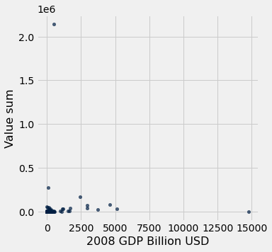
The scatter plot doesn’t show much because most of the data is in a very tiny part of the graph. It’s hard to tell whether the other points are outliers or part of some trend. In this case, one handy tool is to take the log of each x-value and y-value.
Recall that for a number \(n\), \(log(n) = a\) such \(10^a = n\). Here are some values to illustrate how logarithms work:
n |
log(n) |
|---|---|
1 |
0 |
10 |
1 |
100 |
2 |
1,000 |
3 |
10,000 |
4 |
100,000 |
5 |
1,000,000 |
6 |
10,000,000 |
7 |
100,000,000 |
8 |
1,000,000,000 |
9 |
joined.scatter('2008 GDP Billion USD', 'Value sum')
plots.xscale('log')
plots.yscale('log')
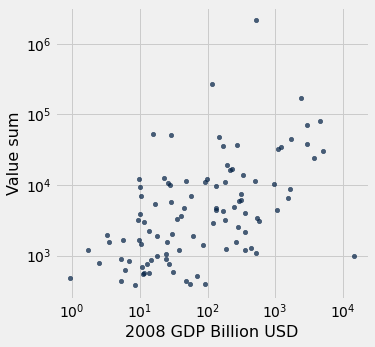
That makes the points more evenly distributed across both axes of the plots, and it makes any correlation jump out. We can do a lot with log-log plots like this, but for us, we will be happy to just use it to make the correlation more apparent in this one example.
What about the relationship between oil production and gift values? You can find oil production for every country or region of the world here.
# Compute the average oil production during the years 2009-2016.
oil = Table().read_table('data/oil_production_by_country.csv')
oil_for_years = oil.where('Year', are.between_or_equal_to(2009, 2016))
oil_by_entity = oil_for_years.drop('Code', 'Year').group('Entity', np.average)
oil_by_entity.sort('Oil production (TWh) average', descending=True)
oil_by_entity.sample(10)
| Entity | Oil production (TWh) average |
|---|---|
| North Korea | 0 |
| Senegal | 0 |
| Turkey | 30.1689 |
| Fiji | 0 |
| Mozambique | 0 |
| United Kingdom | 582.954 |
| Liberia | 0 |
| Kuwait | 1660.07 |
| Guadeloupe | 0 |
| Thailand | 193.364 |
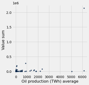
joined_oil = gifts_by_country.join('Country', oil_by_entity, 'Entity')
joined_oil.scatter('Oil production (TWh) average', 'Value sum')
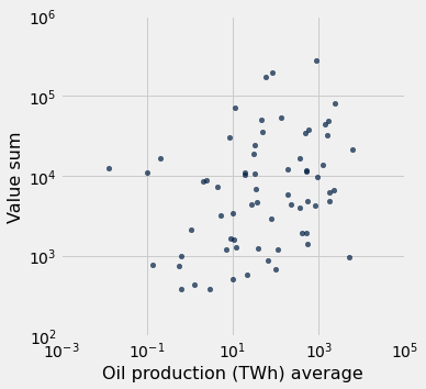
joined_oil.scatter('Oil production (TWh) average', 'Value sum')
plots.xscale('log')
plots.yscale('log')
plots.xlim(1/1e3, 1e5)
plots.ylim(1e2, 1e6);
#If you're curious about the top oil producers in the world...
joined_oil.sort('Oil production (TWh) average', descending=True)
| Country | Value sum | Oil production (TWh) average |
|---|---|---|
| Russia | 21474 | 6153.07 |
| Saudi Arabia | 2.14279e+06 | 6151.13 |
| United States | 974 | 5059.72 |
| China | 79786.5 | 2381.96 |
| Canada | 6541.36 | 2190.7 |
| United Arab Emirates | 6125 | 1825.73 |
| Iraq | 4755.99 | 1819.56 |
| Kuwait | 48265 | 1660.07 |
| Mexico | 32546.2 | 1612.68 |
| Brazil | 44409.7 | 1374.56 |
... (102 rows omitted)
Q: Brainstorm some alternative variables we might want to examine correlations between?
Norms of gift giving? Political alliances? Trade deals?
Could we track if this relationship changes over time?
In this class, we’re going to be moving towards some more of these open-ended data questions.