from datascience import *
import numpy as np

%matplotlib inline
import matplotlib.pyplot as plots
plots.style.use('fivethirtyeight')
Functions
1. Overlaid Histograms
In late 1800s Francis Galton recorded the heights of 930 children who had reached adulthood and the height of their parents. What does the data show?
galton = Table.read_table('data/galton.csv')
galton.show(4)
| family | father | mother | midparentHeight | children | childNum | gender | childHeight |
|---|---|---|---|---|---|---|---|
| 1 | 78.5 | 67 | 75.43 | 4 | 1 | male | 73.2 |
| 1 | 78.5 | 67 | 75.43 | 4 | 2 | female | 69.2 |
| 1 | 78.5 | 67 | 75.43 | 4 | 3 | female | 69 |
| 1 | 78.5 | 67 | 75.43 | 4 | 4 | female | 69 |
... (930 rows omitted)
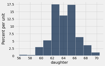
Let’s focus on the female adult children first.
heights = galton.where('gender', 'female').select('father', 'mother', 'childHeight').relabeled(2, 'daughter')
heights
| father | mother | daughter |
|---|---|---|
| 78.5 | 67 | 69.2 |
| 78.5 | 67 | 69 |
| 78.5 | 67 | 69 |
| 75.5 | 66.5 | 65.5 |
| 75.5 | 66.5 | 65.5 |
| 75 | 64 | 68 |
| 75 | 64 | 67 |
| 75 | 64 | 64.5 |
| 75 | 64 | 63 |
| 75 | 58.5 | 66.5 |
... (443 rows omitted)
heights.hist('daughter')
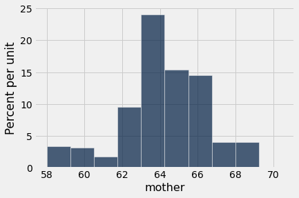
heights.hist('mother')
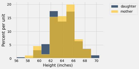
Recall, we can use overlaid histograms to compare the distribution of two variables that have the same units. (Note: We’ve seen how to group by a column containing a categorical. It’s also possible to just call hist with multiple column names to produce an overlaid histogram.)
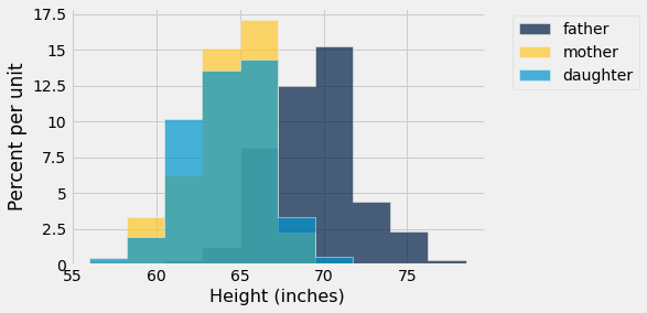
heights.hist('daughter', 'mother')
plots.xlabel('Height (inches)');
heights.hist()
plots.xlabel('Height (inches)');
We can specify bins ourselves to make them have a different width and number.
our_bins = np.arange(55, 81, 1)
print("bins=", our_bins)
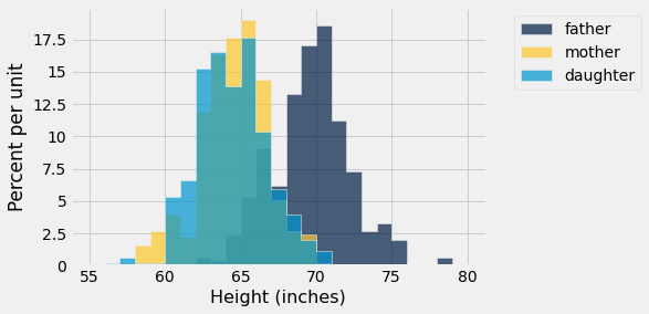
heights.hist(bins=np.arange(55, 81, 1))
plots.xlabel('Height (inches)');
bins= [55 56 57 58 59 60 61 62 63 64 65 66 67 68 69 70 71 72 73 74 75 76 77 78
 79 80]
Let’s now take a different slice of the original data
galton.show(3)
| family | father | mother | midparentHeight | children | childNum | gender | childHeight |
|---|---|---|---|---|---|---|---|
| 1 | 78.5 | 67 | 75.43 | 4 | 1 | male | 73.2 |
| 1 | 78.5 | 67 | 75.43 | 4 | 2 | female | 69.2 |
| 1 | 78.5 | 67 | 75.43 | 4 | 3 | female | 69 |
... (931 rows omitted)
heights = galton.select('father', 'mother', 'childHeight').relabeled(2, 'child')
heights
| father | mother | child |
|---|---|---|
| 78.5 | 67 | 73.2 |
| 78.5 | 67 | 69.2 |
| 78.5 | 67 | 69 |
| 78.5 | 67 | 69 |
| 75.5 | 66.5 | 73.5 |
| 75.5 | 66.5 | 72.5 |
| 75.5 | 66.5 | 65.5 |
| 75.5 | 66.5 | 65.5 |
| 75 | 64 | 71 |
| 75 | 64 | 68 |
... (924 rows omitted)
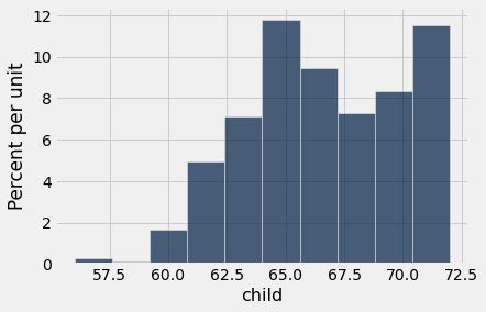
heights.hist(bins=np.arange(55,80,2))
plots.xlabel('Height (inches)');
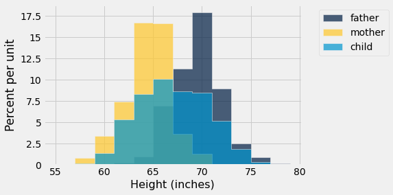
Question: Why is the maximum height of a bar for child smaller than that for mother or father?
A: We have a larger spread because we have both male and female children.
2. Functions
We use functions all the time. They do computation for us without us describing every single step. That saves us time – we don’t have to write the code – and let’s us perform those operations without even caring how they are implemented. Example: max: we have an idea of how we’d take the maximum of a list of numbers, but we can just use that function in Python without explicitely describing how it works.
Can we do the same for other computations? Yes! It’s a core principle of programming: define functions for tasks you do often so you never have to repeat writing the code.
Defining and calling our own functions
def double(x):
    """ Double x """
    return 2*x
double(5)
10
double(double(5))
20
Scoping: parameter only “visible” inside the function definition
x #should throw an error
---------------------------------------------------------------------------
NameError                                 Traceback (most recent call last)
/var/folders/md/kwd9nc_d2ns0hw9wsvdrnt2c0000gn/T/ipykernel_78712/51907093.py in <module>
----> 1 x #should throw an error

NameError: name 'x' is not defined
double(5/4)
2.5
y = 5
double(y/4)
2.5
x
---------------------------------------------------------------------------
NameError                                 Traceback (most recent call last)
/var/folders/md/kwd9nc_d2ns0hw9wsvdrnt2c0000gn/T/ipykernel_78712/32546335.py in <module>
----> 1 x

NameError: name 'x' is not defined
x = 1.5
double(x)
3.0
x
1.5
What happens if I double an array?
double(make_array(3,4,5))
array([ 6, 8, 10])
What happens if I double a string?
double("string")
'stringstring'
5*"string"
'stringstringstringstringstring'
More functions
Think-pair-share:
What is this function below doing?
How would you rewrite this function (the name of the function, the docstring, the parameters) in order to make it more clear?
def f(s):
    total = sum(s)
    return np.round(s / total * 100, 2)
A: Always use meaningul names.
def percents(counts):
    """Convert the counts to percents out of the total."""
    total = sum(counts)
    return np.round(counts / total * 100, 2)
Note that we have a local variable total in our definition….
f(make_array(2, 4, 8, 6, 10))
array([ 6.67, 13.33, 26.67, 20. , 33.33])
percents(make_array(2, 4, 8, 6, 10))
array([ 6.67, 13.33, 26.67, 20. , 33.33])
Remember scoping here too!
total
---------------------------------------------------------------------------
NameError                                 Traceback (most recent call last)
/var/folders/md/kwd9nc_d2ns0hw9wsvdrnt2c0000gn/T/ipykernel_78712/3172011723.py in <module>
----> 1 total

NameError: name 'total' is not defined
Accessing global variables
Global variables are defined outside any function – we’ve been using them all along. You can access global variables that you have defined inside your functions. Always define globals before functions that use them to avoid confusion and surprising results when you rerun your whole notebook!
def children_under_height(height):
    """Proportion of children in our data set that are no taller than the given height."""
    return heights.where("child", are.below_or_equal_to(height)).num_rows / heights.num_rows
children_under_height(65)
0.3747323340471092
Functions with more than one parameter
We can add functions with more than one parameter.
#original function
def percents(counts):
    """Convert the counts to percents out of the total."""
    total = sum(counts)
    return np.round(counts / total * 100, 2)
#function with two parameters
def percents_two_params(counts, decimals_to_round):
    """Convert the counts to percents out of the total."""
    total = sum(counts)
    return np.round(counts / total * 100, decimals_to_round)
counts = make_array(2, 4, 8, 6, 10)
percents(counts)
array([ 6.67, 13.33, 26.67, 20. , 33.33])
percents_two_params(counts, 2)
array([ 6.67, 13.33, 26.67, 20. , 33.33])
percents_two_params(counts, 1)
array([ 6.7, 13.3, 26.7, 20. , 33.3])
percents_two_params(counts, 0)
array([ 7., 13., 27., 20., 33.])
percents_two_params(counts, 3)
array([ 6.667, 13.333, 26.667, 20. , 33.333])
Let’s write a function that given the unique id of an observation (a row) gives us the value of a particular column.
heights_id = heights.with_columns('id', np.arange(heights.num_rows))
heights_id.show(5)
| father | mother | child | id |
|---|---|---|---|
| 78.5 | 67 | 73.2 | 0 |
| 78.5 | 67 | 69.2 | 1 |
| 78.5 | 67 | 69 | 2 |
| 78.5 | 67 | 69 | 3 |
| 75.5 | 66.5 | 73.5 | 4 |
... (929 rows omitted)
def find_a_value(table, observation_id, column_name):
    return table.where('id', are.equal_to(observation_id)).column(column_name).item(0)
find_a_value(heights_id, 2, 'mother')
67.0
find_a_value(heights_id, 200, 'mother')
63.0
Great! Now we can keeping using a function we wrote throughout this class to speed up work in the same way we’re using functions built-in to Python, e.g. max, or the datascience package, e.g. .take()
3. Apply
There are times we want to perform mathematical operations columns of the table but can’t use array broadcasting…
# There are times we want to perform mathetmatical operations columns of the table but can't use array broadcasting
min(make_array(70, 73, 69), 72) #should be an error
---------------------------------------------------------------------------
ValueError                                Traceback (most recent call last)
/var/folders/md/kwd9nc_d2ns0hw9wsvdrnt2c0000gn/T/ipykernel_78712/1957825696.py in <module>
      1 # There are times we want to perform mathetmatical operations columns of the table but can't use array broadcasting
----> 2 min(make_array(70, 73, 69), 72) #should be an error

ValueError: The truth value of an array with more than one element is ambiguous. Use a.any() or a.all()
def cut_off_at_72(x):
    """The smaller of x and 72"""
    return min(x, 72)
cut_off_at_72(62)
62
cut_off_at_72(72)
72
cut_off_at_72(78)
72
The table apply method applies a function to every entry in a column.
heights
| father | mother | child |
|---|---|---|
| 78.5 | 67 | 73.2 |
| 78.5 | 67 | 69.2 |
| 78.5 | 67 | 69 |
| 78.5 | 67 | 69 |
| 75.5 | 66.5 | 73.5 |
| 75.5 | 66.5 | 72.5 |
| 75.5 | 66.5 | 65.5 |
| 75.5 | 66.5 | 65.5 |
| 75 | 64 | 71 |
| 75 | 64 | 68 |
... (924 rows omitted)
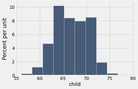
heights.hist('child')
cut_off = heights.apply(cut_off_at_72, 'child')
height2 = heights.with_columns('child', cut_off)
height2.hist('child')
Like we did with variables, we can call functions and their types. In Python, help prints out the docstring of a function.
cut_off_at_72
<function __main__.cut_off_at_72(x)>
type(cut_off_at_72)
function
help(cut_off_at_72)
Help on function cut_off_at_72 in module __main__:

cut_off_at_72(x)
    The smaller of x and 72
Apply with multiple columns
heights.show(6)
| father | mother | child |
|---|---|---|
| 78.5 | 67 | 73.2 |
| 78.5 | 67 | 69.2 |
| 78.5 | 67 | 69 |
| 78.5 | 67 | 69 |
| 75.5 | 66.5 | 73.5 |
| 75.5 | 66.5 | 72.5 |
... (928 rows omitted)
parent_max = heights.apply(max, 'mother', 'father')
parent_max.take(np.arange(0, 6))
array([78.5, 78.5, 78.5, 78.5, 75.5, 75.5])
def average(x, y):
    """Compute the average of two values"""
    return (x+y)/2
parent_avg = heights.apply(average, 'mother', 'father')
parent_avg.take(np.arange(0, 6))
array([72.75, 72.75, 72.75, 72.75, 71. , 71. ])
Left off 2022-09-28
4. Prediction
We’re following the example in Ch. 8.1.3
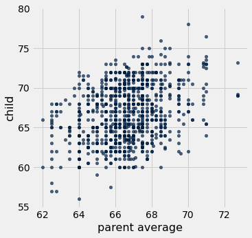
Q: Can we use the average of a child’s parents’ heights to predict the child’s height?
heights.show(10)
| father | mother | child |
|---|---|---|
| 78.5 | 67 | 73.2 |
| 78.5 | 67 | 69.2 |
| 78.5 | 67 | 69 |
| 78.5 | 67 | 69 |
| 75.5 | 66.5 | 73.5 |
| 75.5 | 66.5 | 72.5 |
| 75.5 | 66.5 | 65.5 |
| 75.5 | 66.5 | 65.5 |
| 75 | 64 | 71 |
| 75 | 64 | 68 |
... (924 rows omitted)
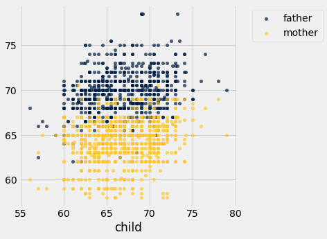
Another scatter plot (Note: Usually we create scatter plot by specifyin two columns: one for x-values and one for y-values, and use a categorical column to group points by color when creating an overlay. If we have a table where we have two columns for y-values that share the same column for x-values, we can create an overlay plot just by specifying the column containing those shared x-values.)
heights.scatter('child')
Add a column with parents’ average height to the height table
heights = heights.with_column(
    'parent average', parent_avg
)
heights
| father | mother | child | parent average |
|---|---|---|---|
| 78.5 | 67 | 73.2 | 72.75 |
| 78.5 | 67 | 69.2 | 72.75 |
| 78.5 | 67 | 69 | 72.75 |
| 78.5 | 67 | 69 | 72.75 |
| 75.5 | 66.5 | 73.5 | 71 |
| 75.5 | 66.5 | 72.5 | 71 |
| 75.5 | 66.5 | 65.5 | 71 |
| 75.5 | 66.5 | 65.5 | 71 |
| 75 | 64 | 71 | 69.5 |
| 75 | 64 | 68 | 69.5 |
... (924 rows omitted)
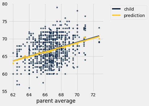
heights.scatter('parent average', 'child')
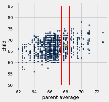
Let’s look at just a subset of the data for illustration.
Think-pair-share: Suppose researchers encountered a new couple, similar to those in this dataset, and wondered how tall their child would be. What would be a good way to predict the child’s height, given that the parent average height was, say, 68 inches (the gold dot below)?
heights.scatter('parent average', 'child')

# this code draws two red lines on the plot to show
# children whose parents' average heights are around 68
_ = plots.plot([67.5, 67.5], [50, 85], color='red', lw=2)
_ = plots.plot([68.5, 68.5], [50, 85], color='red', lw=2)
plots.scatter(68, 67.62, color='gold', s=40);
Let’s look at values around the parents average height and compute a mean child height.
close_to_68 = heights.where('parent average', are.between(67.5, 68.5))
close_to_68
| father | mother | child | parent average |
|---|---|---|---|
| 74 | 62 | 74 | 68 |
| 74 | 62 | 70 | 68 |
| 74 | 62 | 68 | 68 |
| 74 | 62 | 67 | 68 |
| 74 | 62 | 67 | 68 |
| 74 | 62 | 66 | 68 |
| 74 | 62 | 63.5 | 68 |
| 74 | 62 | 63 | 68 |
| 74 | 61 | 65 | 67.5 |
| 73.2 | 63 | 62.7 | 68.1 |
... (175 rows omitted)
close_to_68.column('child').mean()
67.62
Ooo! A function to compute that child mean height for any parent average height
def predict_child(parent_avg_height):
    close_points = heights.where('parent average', are.between(parent_avg_height - 0.5, parent_avg_height + 0.5))
    return close_points.column('child').mean()
predict_child(68)
67.62
predict_child(65)
65.83829787234043
Apply predict_child to all the parent averages.
height_pred = heights.with_column(
    'prediction', heights.apply(predict_child, 'parent average')
)
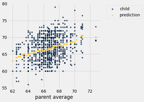
Scatter plot with our predictions. (Note: the child and prediction columns are the y-values, and they share the common x-values in ‘parent average’.
height_pred.select('child', 'parent average', 'prediction').scatter('parent average')
Add a trendline to see how accurate our predictions are…
height_pred.select('child', 'parent average', 'prediction').scatter('parent average', fit_line=True)