Lab 2: Thrown for a Loop: Monte Carlo Methods
This labs explores iteration and how it can be used to abstract away repetitive tasks in a clean and consise way. In addition, it highlights a monte carlo method for estimating π and, for extra credit, a monte carlo method for estimating e.
Step 1: Source Code
This week we will use the sanbox method for code deployment and collection. You should find a repository in the williams-cs organization called <git-username>-lab2. This repo is accessible only to you, the instructor, and the teaching assistants. Because of this, you will not need to fork it, only clone it to your local disk.
- Clone your private repo to an appropriate directory in your home folder
(
~/labsis a good choice):$ git clone https://github.com/<git-username>/lab2.git
Remember, you can always get the repo address by using the https copy-to-clipboard link on github. - Once inside your <git-username>-lab2 directory,
create a virtual environment using:
$ virtualenv -p python3 venv
- Activate your environment by typing:
$ . venv/bin/activate
- Remember that you must always activate your virtual environment when opening a new terminal
- Type
$ git branch
and notice that you are currently editing the master branch. - Create a new branch with
$ git branch loop
This branch is represents a split from the master branch. - Checkout this branch by typing
$ git checkout loop
- Any changes you make to the repository are now isolated on this branch.
Step 1: Practice Looping
Consider the following python program
called pattern_a.py (it's provided in the source
code) that accepts an integer argument and produces the following
output.
pattern_a.py <num>
    $ python3 pattern_a.py 3

    1 1 1
    2 2 2
    3 3 3

    $ python3 pattern_a.py 4

    1 1 1 1
    2 2 2 2
    3 3 3 3
    4 4 4 4

    $ python3 pattern_a.py 5

    1 1 1 1 1
    2 2 2 2 2
    3 3 3 3 3
    4 4 4 4 4
    5 5 5 5 5
Write four different python programs called pattern_b.py, pattern_c.py,
pattern_n.py, and pattern_z.py respectively.
Each program takes a single positive integer assignment and
produces the correctly formatted output, examples of which are
given below. Remember that you can surpress
the newline character at the end of the print
function by using the optional final
argument end. Here is an example: print("some string", end="").
Pattern B
pattern_b.py <num>
produces the following output when called with appropriate integer argument.
    $ python3 pattern_b.py 3

    1 2 3
    2 3
    3

    $ python3 pattern_b.py 4

    1 2 3 4
    2 3 4
    3 4
    4

    $ python3 pattern_b.py 5

    1 2 3 4 5
    2 3 4 5
    3 4 5
    4 5
    5
By default, any file you create is not included in your repository. To ensure that you can work on your code anywhere, it's important to both add your code to your repository, to commit your changes to the repository, and to push your changes back up to github. Let's practice here.
- First, add the pattern_b.py file to your local repo.
$ git add pattern_b.py
- Second, commit your changes to the repo.
$ git commit -m 'inital commit of pattern b' -a
The -m flag is the commit message, which appears in the commit log. The -a flag says commit all files that have changed since the last commit. - Finally, push your changes back to github.
$ git push
You will probably be asked to type:$ git push --set-upstream origin loop
which you should do. This pushes your loop branch back up to the GitHub Repo.
Pattern C
pattern_c.py <num>
produces the following output when called with appropriate integer argument.
    $ python3 pattern_c.py 3

    1
    1 2 2
    1 2 2 3 3 3

    $ python3 pattern_c.py 4

    1
    1 2 2
    1 2 2 3 3 3
    1 2 2 3 3 3 4 4 4 4

    $ python3 pattern_c.py 5

    1
    1 2 2
    1 2 2 3 3 3
    1 2 2 3 3 3 4 4 4 4
    1 2 2 3 3 3 4 4 4 4 5 5 5 5 5
Pattern N
pattern_n.py <num>
produces the following output when called with appropriate integer argument.
    $ python3 pattern_n.py 2

    *  *
    ** *
    * **
    *  *

    $ python3 pattern_n.py 3

    *   *
    **  *
    * * *
    *  **
    *   *

    $ python3 pattern_n.py 4

    *    *
    **   *
    * *  *
    *  * *
    *   **
    *    *
Pattern Z
pattern_z.py <num>
produces the following output when called with appropriate integer argument.
    $ python3 pattern_z.py 2

    ****
      *
     *
    ****

    $ python3 pattern_z.py 3

    *****
       *
      *
     *
    *****

    $ python3 pattern_z.py 4

    ******
        *
       *
      *
     *
    ******
Step 2: Monte Carlo Methods
Here's a cool way to estimate π: throw a bunch darts at dartboard with radius
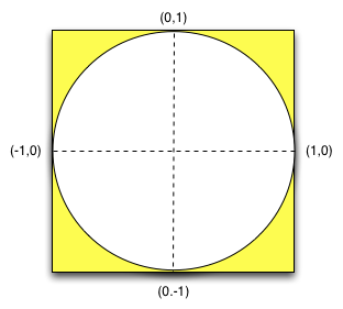
The dartboard has area π × r2=π and the case has area 4, so if your throws are uniformly distributed inside the case, then the ratio of darts hitting the dart board to the dart case should be π/4. Multiplying this ratio by 4 gives you an estimate of π.
Use the random
module (and specifically the
function random.uniform(a,b)) to simulate the dart
throwing.
Implement the following functions (hint: calculate_pi
should call both rand() and distance) and
test your code with increasing sample sizes (you should see more
accurate estimates of π)
    def rand():
        """return a number uniformly at random in the range [-1,1]"""
     def distance(x,y):
	 """return the euclidean distance between (0,0) and (x,y)"""
     def calculate_pi(n):
	 """
	 Calculate PI by comparing the ratio of points landing
	 in the circle with radius 1 to those landing outside
	 """
    $ python3 pi.py 10
    2.8

    $ python3 pi.py 100
    3.28

    $ python3 pi.py 1000
    3.232

    $ python3 pi.py 10000
    3.1524

    $ python3 pi.py 100000
    3.13804

    $ python3 pi.py 1000000
    3.14012
Extra-Credit: Estimating e
The mathematical constant e
plays a pivotal role in
mathematics. It is approximately
2.718. One way to approximate the
number is to use computer-intensive
monte carlo methods, like we did
with estimating π. Here's how,
imagine you have an infinite list
of random numbers
The file e.py contains headers for two
functions estimate and sample.
Implement these functions.
     import random
     import sys

     def estimate():
        """
        One estimate of the constant 'e' involves generaing an infinite sequence
        of random numbers in the range (0,1). Call these values X1, X2, X3, ...
        The smallest value n such that the sum of X1 + X2 + ... + Xn > 1 gives
        an estimate for 'e'.  This function returns one such estimate.  In other
        words, it repeatedly generates numbers in the range (0,1), adding them to
        a total, and returns the number of iterations after which the total first
        exceeds 1"""

     def sample(n):
        """
        Return the average estimate() value over n samples.
        As n increases, this gives an increasingly more accurate estimate
        of the constant 'e'"""

     print(sample(int(sys.argv[1])))
      $ python3 e.py 10
      2.8

      $ python3 e.py 100
      2.6

      $ python3 e.py 1000
      2.704

      $ python3 e.py 10000
      2.7244

      $ python3 e.py 100000
      2.72335

      $ python3 e.py 1000000
      2.718798

      $ python3 e.py 10000000
      2.7180784
Step 4: Submission
- When you cloned your private repo locally, it contained the following four files:
- README.md
- e.py
- pattern_a.py
- pi.py
- You can verify that there aren't any outstanding changes waiting to be committed by typing
$ git status
- Finally, push your changes back to github repo:
$ git push - When you're ready to submit this code to us, issue a pull request by going to githb and clicking on the green Compare & pull request button.
Credit
The looping problems come from Tom Wexler and the dartboard example for the monte carlo problem for estimating π comes from Alexa Sharp